
Predicting House Prices
All the files of this project are saved in a GitHub repository.
King County House Sales Dataset
The King County House Sales dataset contains the house sales around Seattle, in King County (USA), between May 2014 and May 2015. The original dataset can be found on Kaggle.
The dataset consists in:
- Train Set with 17,277 observations with 19 house features, the ID, and the price.
- Test Set with 4,320 observations with 19 house features and the
ID. The
pricecolumn will be added to the Test Set, with NAs, to ease the pre-processing stage.
This map shows where the properties listed in the dataset are located:
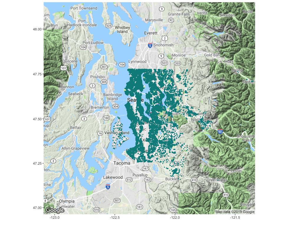
This project aims to predict house prices based on their features.
Packages
This analysis requires these R packages:
- Data Manipulation:
data.table,dplyr,tibble,tidyr - Plotting:
corrplot,GGally,ggmap,ggplot2,grid,gridExtra - Machine Learning:
caret,dbscan,glmnet,leaderCluster,MLmetrics,ranger,xgboost - Multithreading:
doMC,doParallel,factoextra,foreach,parallel - Reporting:
kableExtra,knitr,RColorBrewer,shiny, and…beepr.
These packages are installed and loaded if necessary by the main script.
Data Loading
The dataset is pretty clean, with no missing value in both Train and
Test sets. A quick look at the id values also shows that only a few
houses have been sold more than once on the period, so it doesn’t seem
relevant the consider the id and the date for this analysis. We will
thus focus on the house features to predict its price.
## [1] "0 columns of the Train Set have NAs."
## [1] "0 columns of the Test Set have NAs."
## [1] "103 houses sold more than once on the period, for a total of 17173 houses in the Train Set (0.006%)."
## [1] "8 houses in the Test Set sold more than once on the period, for a total of 4312 houses in the Test Set (0.002%)."
Some of the features can be converted into factors, as they are not continuous and help categorizing the house:
waterfrontis a boolean, indicating if the house has a view to a waterfront.viewindicated the number of times the house has been viewed. As it only has 4 values, this feature can be factorized.conditionis a score from 1 to 5, indicating the state of the house.gradeis another score, with 11 levels.bedroomsis typically used to categorize houses.
The package caret automatically one-hot encodes the categorical
features when fitting a model. Due to their number of unique values,
these features won’t be factorized at first:
bathroomscould also be used to categorize the houses, although it is not clear why the data shows decimal numbers.zipcodeis a cluster-like category of the house location.
The impact of processing them as factors will be tested with a Linear Regression.
Exploratory Data Analysis
The target of this analysis is the price of the houses. Like the real
estate market, the price variable is highly right-skewed, with its
maximum value being more than 10 times larger than the 3rd quartile:
##    Min. 1st Qu.  Median    Mean 3rd Qu.    Max.
##   78000  320000  450000  539865  645500 7700000
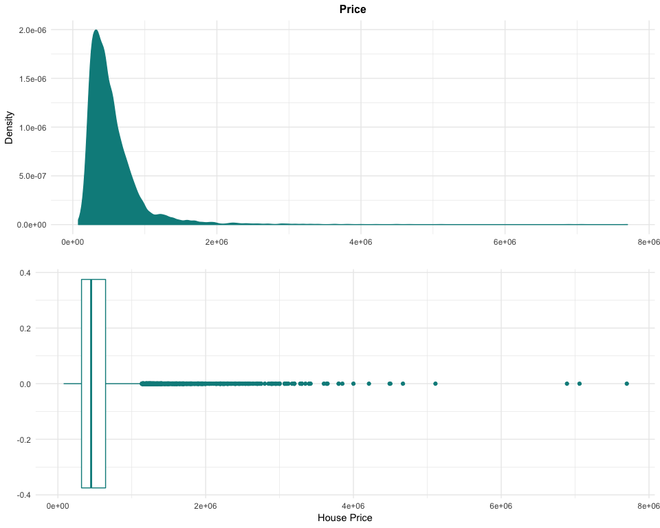
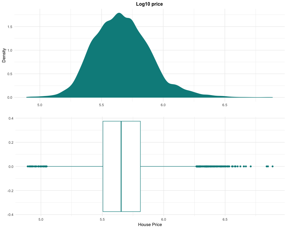
These properties of high-value cannot be removed from the dataset, as they are not anomalies but examples of the luxury market in the region. By transforming the data with a logarithm to base 10, it is possible to easily rebalance the dataset. This transformation could be used later to try to improve our models’ performance.
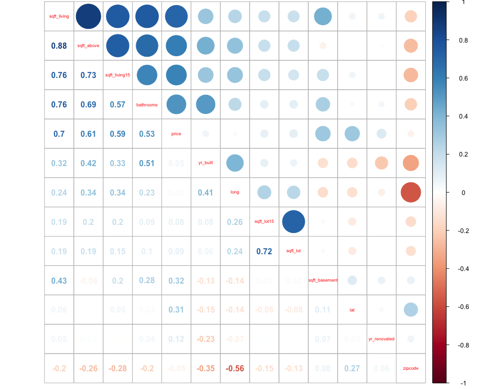
The Correlation Matrix between the numerical features of the Train Set
indicates some correlation between the price and:
sqft_living: more living area logically implies a higher price.sqft_living15: the living area in 2015 is also linked to the current price. Recent renovations have modified the living area, but it is likely that the house stays in a similar price range.sqft_above: by definition, the area above ground is related to the living area. It is not a surprice to see correlation with the price as well.bathrooms: interestingly, the number of bathrooms seems to slightly correlate with the price.
Some other relationships can be identified:
- the
sqft_features are linked to each others, assqft_living = sqft_above + sqft_basement, and the lot areas are usually not changing much within a year. - the
zipcodeand thelongitude are quite linked, maybe due to the way zipcode have been designed in the region.
This other Correlation Matrix provides another view of the relationship between features, as well as their own distribution.

The following charts allow to understand the structure of each factor feature:
- A majority of houses in the region have 3 or 4 bedrooms. An overall trend shows that more bedrooms means higher prices.
- Most of the houses in the region are in an average condition
3, with 26% of the houses being in a great condition4, and 8% being in an exceptional condition5. - The real estate market in the region seems to offer almost as many houses with two floors than with one floor.
- The grade distribution is similar than the condition (with more levels), but the relation to price looks clearer.
- Houses with more views seem to be in a higher price range.
- Houses with a view the waterfront are clearly more expensive than the ones without.
The following charts describe the numercial features and provide interesting insights:
- The number of
bathroomsis difficult to interpret without knowing the meaning of the decimals. But it seems that majority of houses have values of 2.5 and 1. - The latitude and longitude distributions suggest a higher number of properties in the North-West of the region.
- The floor space is also right-skewed, with a large portion of the houses having no basement.
- Looking at the distribution of the feature
yr_built, we can observe a regular increase of real estate projects since the early years of the 20th century. This trend can certainly be related to the population growth and the urban development in the region over the years. - With only 739 properties with renovation records, the
yr_renovatedfeature is extremely right-skewed. If we consider only the properties with records, renovations go from 1934 till 2015, with higher numbers from the 80s, and a big wave of renovations in 2013 and 2014. - Houses in the dataset seem quite well distributed across the
zipcoderange, although it is difficult to comment this feature without a good knowlegde of the region and the structure of the zipcode system.
Data Preparation
As the Test Set doesn’t contain the feature price, it is necessary to
randomly split the Train Set in two, with a 80|20 ratio:
- Train Set A, which will be used to train our model.
- Train Set B, which will be used to test our model and validate the performance of the model.
These datasets are centered and scaled, using the preProcess function
of the package caret. These transformations should improve the
performance of linear models.
Copies of these datasets are prepared with the features bathrooms and
zipcode set as factors, and other copies with the price being
transformed with log10. These versions of the datasets will allow to
test the response of our models to different inputs.
Cross-Validation Strategy
To validate the stability of our models, we will apply a 10-fold cross-validation, repeated 3 times.
Baseline
At first, we use the linear regression algorithm to fit models on different dataset configurations:
- The prepared datasets, without additional transformation,
- The prepared datasets with
pricebeing transformed with log10, - The prepared datasets with
bathroomsandzipcodeas factors, - The prepared datasets with both transformations.
| model | RMSE | Rsquared | MAE | MAPE | Coefficients | Train Time (min) |
|---|---|---|---|---|---|---|
| Baseline Lin. Reg. | 173375.7 | 0.7371931 | 115993.74 | 0.2340575 | 48 | 0.1 |
| Baseline Lin. Reg. Log | 167660.5 | 0.7542339 | 106380.01 | 0.1987122 | 48 | 0.1 |
| Baseline Lin. Reg. All Fact | 132157.4 | 0.8472985 | 85342.24 | 0.1702119 | 143 | 0.3 |
| Baseline Lin. Reg. Log All Fact | 126177.3 | 0.8608053 | 74064.56 | 0.1394403 | 143 | 0.3 |
The two transformations appear to improve the performance of the model,
both individually and jointly. The log10 helps by centering the ‘price’
and reduce the influence of high values. The class change of bathrooms
and zipcode avoids the model to consider them as ordinal features,
which is particularly useful for zipcode which characterizes house
clusters.
We continue by training models with a random forest using the
package ranger, then with an eXtreme Gradient BOOSTing (XGBoost),
both on the four possible combinations of
transformations.
| RMSE | Rsquared | MAE | MAPE | Coefficients | Train Time (min) | |
|---|---|---|---|---|---|---|
| Baseline Lin. Reg. | 173375.7 | 0.7371931 | 115993.74 | 0.2340575 | 48 | 0.1 |
| Baseline Lin. Reg. Log | 167660.5 | 0.7542339 | 106380.01 | 0.1987122 | 48 | 0.1 |
| Baseline Lin. Reg. All Fact | 132157.4 | 0.8472985 | 85342.24 | 0.1702119 | 143 | 0.3 |
| Baseline Lin. Reg. Log All Fact | 126177.3 | 0.8608053 | 74064.56 | 0.1394403 | 143 | 0.3 |
| Baseline Ranger | 117953.9 | 0.8783576 | 68898.26 | 0.1357399 | 47 | 26.3 |
| Baseline Ranger Log | 122706.6 | 0.8683575 | 69140.95 | 0.1306257 | 47 | 26.0 |
| Baseline Ranger All Fact | 114785.7 | 0.8848043 | 67552.36 | 0.1330712 | 142 | 123.5 |
| Baseline Ranger Log All Fact | 118612.8 | 0.8769947 | 67751.38 | 0.1281304 | 142 | 122.1 |
| Baseline XGBoost | 116039.2 | 0.8822746 | 71617.33 | 0.1427542 | 47 | 11.8 |
| Baseline XGBoost Log | 110893.0 | 0.8924851 | 67756.69 | 0.1307163 | 47 | 11.1 |
| Baseline XGBoost All Fact | 110899.7 | 0.8924722 | 69604.63 | 0.1394589 | 142 | 33.5 |
| Baseline XGBoost Log All Fact | 109891.8 | 0.8944177 | 66483.14 | 0.1287528 | 142 | 29.3 |
These results confirm our previous conclusions:
- the log10 transformation has a great impact on the model performance. It will be kept for next models.
- the class change of
bathroomsandzipcodehas lower impact, but still improves the results.
Looking at the algorithm performances, Ranger has slighlty better results than XGBoost, but the calculation time being significantly longer for Ranger, we will continue with XGBoost only.
Feature Engineering
House Age and Renovation
A few features can be developped, focusing on the yr_built and
yr_renovated of the house:
house_age: the difference between theyr_builtand 2015 gives the age of the house.house_age_since_renovation: the difference between theyr_renovatedand 2015 indicates since how many years the house hasn’t been renovated.renovated: a boolean flag indicating if the house has been renovated at least once.
Clusters
Another element which might influence the price of a house is the dynamism of the market in the area. Some neighborhoods are more in demand than others, either because of the price or because of the reputation. Thus, it would be interesting to add a feature that considers the density of house sales in the area.
This hexagonal binning map shows the areas with high density of house sales, which are mainly located in the North-West of the region. Some other hotspots can be found in the eastern area too.
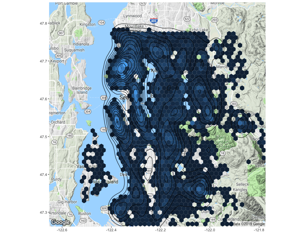
To identify areas of high house sales density, we will use the
clustering algorithm DBSCAN (Density-Based Spatial Clustering of
Application with Noise) from the package dbscan. This algorithm groups
points that are closely packed together, and marks as outliers the
points that lie alone in low-density regions.
This algorithm requires two parameters:
eps- epsilon: defines the radius of neigborhood around a pointx(reachability maximum distance).minPts: defines the minimum number of neighbors within epsilon radius. If the pointxis not surrounded byminPtsneighbors, it is considered as an outlier.
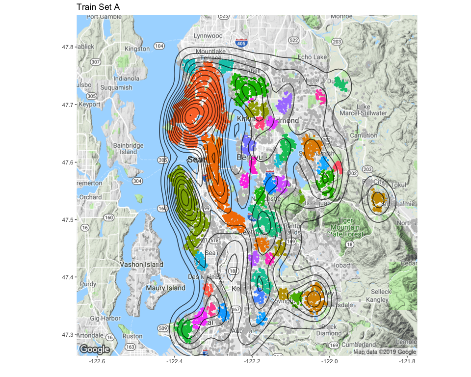
After multiple trials, it appeared that the parameters providing a
maximum number of relevant clusters were eps = 0.0114 and minPts
= 50. This plot shows which areas have been defined as high-density
clusters, using the Train Set
A.
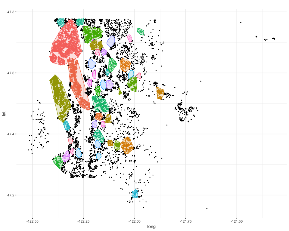
The clusters now being found based on Train Set A, we can asociate them to the points of Train Set B. The maps below allow to compare the results and confirm that the points of Train Set B are assigned to the right cluster.

With these new features, we can train a new model and compare the results with the previous ones.
| RMSE | Rsquared | MAE | MAPE | Coefficients | Train Time (min) | |
|---|---|---|---|---|---|---|
| Baseline Ranger Log | 122706.6 | 0.8683575 | 69140.95 | 0.1306257 | 47 | 26.0 |
| Baseline Ranger Log All Fact | 118612.8 | 0.8769947 | 67751.38 | 0.1281304 | 142 | 122.1 |
| Baseline XGBoost Log All Fact | 109891.8 | 0.8944177 | 66483.14 | 0.1287528 | 142 | 29.3 |
| FE XGBoost | 119055.1 | 0.8760756 | 67999.89 | 0.1299648 | 190 | 40.9 |
The new model obtains a reasonable result, although it didn’t beat the two best models.
Feature Selection with Lasso and RFE
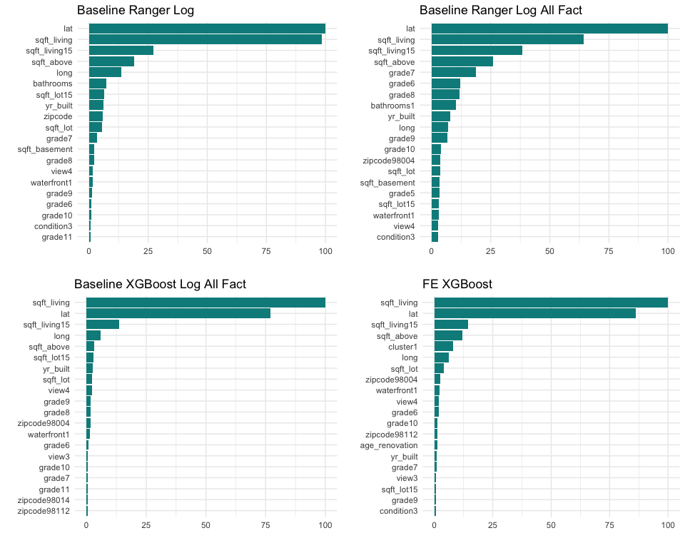
We can compare the Top 20 feature importances for the 4 best models, and observe some similarities:
latandlongappear in all four Top 20, withlathaving a really high importance. It might indicate that the house prices depend a lot on the location on the North-South axis.sqft_livingand its related featuressqft_above,sqft_living15are also at the top of the list, which is not really surprising.gradevalues are important, especially the higher ones. It might indicate that higher grades have a significant impact on the house price.yr_builtusually appears at the first tier of the Top 20s.- As a great indicator of the house location, the
zipcodeseems to have some kind of importance.zipcode98004andzipcode98112in particular appear in the Top 20. These neighborhoods might have specific characteristics which influence the prices. waterfrontappears in the four Top 20, which might be a great add-value for properties in this area.condition3, which indicate that the house in a fair condition, seems to impact the price as well.view4has also an influence on the price. It could indicate lower prices, due to the difficulty to find a buyer. Or in the opposite, it could indicate prices higher than the market. A better look at the models structures will give us better insights.
Lasso Regression
With 190 features, the model resulting from the Feature Engineering stage is quite complex and would benefit from cutting down its number of variables. Also, only a few parameters seem to have a real importance for the model result. Thus, we will start our trimming process with a Lasso Regression which is forcing the coefficients with minor contribution to be equal to 0. We will then get a list of features that we can ignore for our model.
## [1] "The Lasso Regression selected 188 variables, and rejected 12 variables."
| Rejected Features | |||
|---|---|---|---|
| bedrooms.3 | bathrooms.5.5 | view.2 | renovated.0 |
| bathrooms.3 | bathrooms.7.5 | condition.4 | renovated.1 |
| bathrooms.4.5 | waterfront.1 | grade.8 | cluster.10 |
We can note that the new feature renovated has been rejected all
together. Large values of bathrooms also don’t seem to have any impact
on the price.
Recursive Feature Elimination
The dataset being lightened from a few features, we continue the feature selection using a RFE (Recursive Feature Elimination), which will test the variable importances for models trained on subsets with predefined number of variables. This should help to reduce the number of variables with a low impact on the model performance.
For this RFE, we use Random Forest algorithms and 5-fold Cross-Validation. This chart shows the RMSE obtained for each iteration of the RFE.
Note: the RMSE hasn’t been rescaled, which explains the difference with the table of model results.
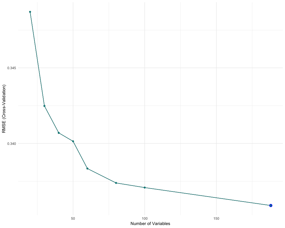
Although we can’t observe any clear ‘knee’, which would indicate that many features could be eliminated with a low impact on the model performance, we could expect to get a fair result for subsets of 40 to 60 features. It is here difficult to estimate the impact on the metrics, as the RMSE shown here is re-scalled.
If we look at the variables importance, we can see that 4 features have a great impact on the model performance, while the importance then decreases slowly to be almost insignificant after the 25th feature.

By defining an arbitrary threshold, we can filter the features with low importance. We decide that features that have an importance less than 0.1% overall should be eliminated. We end up with a list of 37 features which cumulate 96.8% of the variable importances. We can expect a low impact on the model performance, which could be recaptured with model fine tuning.
| Selected Features | ||||
|---|---|---|---|---|
| zipcode.98040 | grade.12 | grade.5 | zipcode.98106 | bedrooms.2 |
| bedrooms.4 | condition.2 | cluster.2 | yr_renovated | cluster.0 |
| zipcode.98112 | floors.2 | cluster.31 | condition.3 | floors.1 |
| view.4 | waterfront.0 | grade.11 | zipcode.98004 | grade.9 |
| grade.6 | grade.10 | age_renovation | sqft_basement | cluster.1 |
| house_age | yr_built | bathrooms.1 | view.0 | sqft_lot |
| sqft_lot15 | grade.7 | long | sqft_above | sqft_living15 |
| sqft_living | lat |
Using this list of selected features, we can re-train an XGBoost model and compare it with previous results.
| model | RMSE | Rsquared | MAE | MAPE | Coefficients | Train Time (min) |
|---|---|---|---|---|---|---|
| Baseline Ranger Log | 122706.6 | 0.8683575 | 69140.95 | 0.1306257 | 47 | 26.0 |
| Baseline Ranger Log All Fact | 118612.8 | 0.8769947 | 67751.38 | 0.1281304 | 142 | 122.1 |
| Baseline XGBoost Log All Fact | 109891.8 | 0.8944177 | 66483.14 | 0.1287528 | 142 | 29.3 |
| FE XGBoost | 119055.1 | 0.8760756 | 67999.89 | 0.1299648 | 190 | 40.9 |
| XGBoost Post RFE | 118315.5 | 0.8776106 | 69053.40 | 0.1323090 | 37 | 9.4 |
The performance of the model post-RFE is not as good as the previous models, but with only 37 features, it is still a very good score! We should be able to catch-up on results with some model tuning.
Tuning
After subsetting the features selected by the Lasso and RFE steps, we proceed to model tuning on a XGBoost and a Ranger, to see which one provides the best results.
Starting with the XGBoost, we use a Tune Grid to fine best combination of parameters.

These charts don’t reveal any opportunity to easily improve the result of the parameters we already tested. Thus, we can approve the best model from this search, which used these parameters:
| nrounds | max_depth | eta | gamma | colsample_bytree | min_child_weight | subsample |
|---|---|---|---|---|---|---|
| 900 | 4 | 0.1 | 0 | 1 | 3 | 1 |
Trying now with a Ranger algorithm, which provided really good results before Feature Engineering.
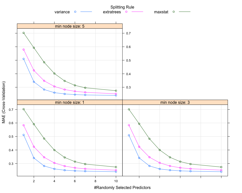
These charts don’t reveal any opportunity to easily improve the result.
We might actually have pushed a bit much on the mtry parameter.
Anyway, we can approve the best model from this search, which used these
parameters:
| mtry | splitrule | min.node.size |
|---|---|---|
| 10 | variance | 1 |
Let’s compare these two new models with the previous best ones.
| model | RMSE | Rsquared | MAE | MAPE | Coefficients | Train Time (min) |
|---|---|---|---|---|---|---|
| Baseline Ranger Log | 122706.6 | 0.8683575 | 69140.95 | 0.1306257 | 47 | 26.0 |
| Baseline Ranger Log All Fact | 118612.8 | 0.8769947 | 67751.38 | 0.1281304 | 142 | 122.1 |
| Baseline XGBoost Log All Fact | 109891.8 | 0.8944177 | 66483.14 | 0.1287528 | 142 | 29.3 |
| FE XGBoost | 119055.1 | 0.8760756 | 67999.89 | 0.1299648 | 190 | 40.9 |
| XGBoost Post RFE | 118315.5 | 0.8776106 | 69053.40 | 0.1323090 | 37 | 9.4 |
| Tuning XGBoost | 112054.8 | 0.8902204 | 64687.33 | 0.1253911 | 37 | 73.3 |
| Tuning Ranger | 121960.2 | 0.8699540 | 69505.40 | 0.1316731 | 37 | 34.2 |
The Tuned XGBoost performs very well, outperforming the previous
records! The Tuned Ranger, on the other hand, is a bit disappointing,
as it is actually worse than the Baseline Ranger with Log10(price)…
Final Model
The best model for this analysis is the Tuned XGBoost, which reaches the MAPE score of 0.1253911 with only 37 features.
| model | RMSE | Rsquared | MAE | MAPE | Coefficients | Train Time (min) |
|---|---|---|---|---|---|---|
| Tuning XGBoost | 112054.8 | 0.8902204 | 64687.33 | 0.1253911 | 37 | 73.3 |
The model uses these parameters:
| nrounds | max_depth | eta | gamma | colsample_bytree | min_child_weight | subsample |
|---|---|---|---|---|---|---|
| 900 | 4 | 0.1 | 0 | 1 | 3 | 1 |
The model needs these features as input:
| Features | ||||
|---|---|---|---|---|
| zipcode.98040 | grade.12 | grade.5 | zipcode.98106 | bedrooms.2 |
| bedrooms.4 | condition.2 | cluster.2 | yr_renovated | cluster.0 |
| zipcode.98112 | floors.2 | cluster.31 | condition.3 | floors.1 |
| view.4 | waterfront.0 | grade.11 | zipcode.98004 | grade.9 |
| grade.6 | grade.10 | age_renovation | sqft_basement | cluster.1 |
| house_age | yr_built | bathrooms.1 | view.0 | sqft_lot |
| sqft_lot15 | grade.7 | long | sqft_above | sqft_living15 |
| sqft_living | lat |
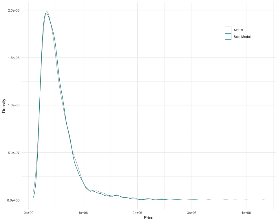
Comparing the predictions of our model with the actual values of the Train Set B would provide an idea of its limitations. We can notice that the model has difficulties to predict prices between 0.75 and 1 million dollars. Further work on Feature Engineering might be able to improve the results in this area.
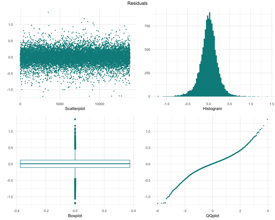
These charts provide different views of the model residuals, which allow to identify possible characteristics of the data which might not be well modeled. We can see that overall, the residuals look normaly distributed, but there might be some possible improvements, as some outliers can be seen on the scatterplot and on the boxplot, and the QQplot displays a ‘wavy’ line insteand of a straight one.
The model now needs to be applied on the Test Set, for which we haven’t the actual prices in this analysis. All the metrics mentioned in this report only apply to the Train Set B. Applying the model on the Test Set will allow to validate if the model is relevant with unknown data.
Annexe - All Models and Results
| model | RMSE | Rsquared | MAE | MAPE | Coefficients | Train Time (min) |
|---|---|---|---|---|---|---|
| Baseline Lin. Reg. | 173375.7 | 0.7371931 | 115993.74 | 0.2340575 | 48 | 0.1 |
| Baseline Lin. Reg. Log | 167660.5 | 0.7542339 | 106380.01 | 0.1987122 | 48 | 0.1 |
| Baseline Lin. Reg. All Fact | 132157.4 | 0.8472985 | 85342.24 | 0.1702119 | 143 | 0.3 |
| Baseline Lin. Reg. Log All Fact | 126177.3 | 0.8608053 | 74064.56 | 0.1394403 | 143 | 0.3 |
| Baseline Ranger | 117953.9 | 0.8783576 | 68898.26 | 0.1357399 | 47 | 26.3 |
| Baseline Ranger Log | 122706.6 | 0.8683575 | 69140.95 | 0.1306257 | 47 | 26.0 |
| Baseline Ranger All Fact | 114785.7 | 0.8848043 | 67552.36 | 0.1330712 | 142 | 123.5 |
| Baseline Ranger Log All Fact | 118612.8 | 0.8769947 | 67751.38 | 0.1281304 | 142 | 122.1 |
| Baseline XGBoost | 116039.2 | 0.8822746 | 71617.33 | 0.1427542 | 47 | 11.8 |
| Baseline XGBoost Log | 110893.0 | 0.8924851 | 67756.69 | 0.1307163 | 47 | 11.1 |
| Baseline XGBoost All Fact | 110899.7 | 0.8924722 | 69604.63 | 0.1394589 | 142 | 33.5 |
| Baseline XGBoost Log All Fact | 109891.8 | 0.8944177 | 66483.14 | 0.1287528 | 142 | 29.3 |
| FE XGBoost | 119055.1 | 0.8760756 | 67999.89 | 0.1299648 | 190 | 40.9 |
| FE XGBoost Clusters | 113018.6 | 0.8883238 | 70184.98 | 0.1397804 | 48 | 13.2 |
| FE XGBoost Clusters Fact | 115534.0 | 0.8832976 | 71665.63 | 0.1415128 | 92 | 22.3 |
| FE XGBoost Clusters All Fact | 114216.9 | 0.8859432 | 70396.77 | 0.1395339 | 187 | 43.9 |
| XGBoost Post RFE | 118315.5 | 0.8776106 | 69053.40 | 0.1323090 | 37 | 9.4 |
| Tuning XGBoost | 112054.8 | 0.8902204 | 64687.33 | 0.1253911 | 37 | 73.3 |
| Tuning Ranger | 121960.2 | 0.8699540 | 69505.40 | 0.1316731 | 37 | 34.2 |