
Human Resources Analytics
All the files of this project are saved in a GitHub repository.
Introduction
Objectives
This case study aims to model the probability of attrition of each employee from the HR Analytics Dataset, available on Kaggle. Its conclusions will allow the management to understand which factors urge the employees to leave the company and which changes should be made to avoid their departure.
Libraries
This project uses a set of libraries for data manipulation, plotting and modelling.
# Loading Libraries
import pandas as pd #Data Manipulation
import numpy as np #Data Manipulation

import matplotlib.pyplot as plt #Plotting
import seaborn as sns #Plotting
sns.set(style='white')

from sklearn import preprocessing #Preprocessing

from scipy.stats import skew, boxcox_normmax #Preprocessing
from scipy.special import boxcox1p #Preprocessing

from sklearn.model_selection import train_test_split #Train/Test Split
from sklearn.linear_model import LogisticRegression #Model

from sklearn.metrics import classification_report #Metrics
from sklearn.metrics import confusion_matrix #Metrics
from sklearn.metrics import accuracy_score #Metrics
from sklearn.metrics import roc_auc_score, roc_curve #ROC
from sklearn import model_selection #Cross Validation
from sklearn.feature_selection import RFE, RFECV #Feature Selection
Data Loading
The dataset is stored in the GitHub repository as a CSV file: turnover.csv. The file is loaded directly from the repository.
# Reading Dataset from GitHub repository
hr = pd.read_csv('https://raw.githubusercontent.com/ashomah/HR-Analytics/master/assets/data/turnover.csv')
hr.head()
| satisfaction_level | last_evaluation | number_project | average_montly_hours | time_spend_company | Work_accident | left | promotion_last_5years | sales | salary | |
|---|---|---|---|---|---|---|---|---|---|---|
| 0 | 0.38 | 0.53 | 2 | 157 | 3 | 0 | 1 | 0 | sales | low |
| 1 | 0.80 | 0.86 | 5 | 262 | 6 | 0 | 1 | 0 | sales | medium |
| 2 | 0.11 | 0.88 | 7 | 272 | 4 | 0 | 1 | 0 | sales | medium |
| 3 | 0.72 | 0.87 | 5 | 223 | 5 | 0 | 1 | 0 | sales | low |
| 4 | 0.37 | 0.52 | 2 | 159 | 3 | 0 | 1 | 0 | sales | low |
Data Preparation
Variables Types and Definitions
The first stage of this analysis is to describe the dataset, understand the meaning of variable and perform the necessary adjustments to ensure that the data will be proceeded correctly during the Machine Learning process.
# Shape of the data frame
print('Rows:', hr.shape[0], '| Columns:', hr.shape[1])
Rows: 14999 | Columns: 10
# Describe each variable
def df_desc(df):
    import pandas as pd
    desc = pd.DataFrame({'dtype': df.dtypes,
                         'NAs': df.isna().sum(),
                         'Numerical': (df.dtypes != 'object') & (df.apply(lambda column: column == 0).sum() + df.apply(lambda column: column == 1).sum() != len(df)),
                         'Boolean': df.apply(lambda column: column == 0).sum() + df.apply(lambda column: column == 1).sum() == len(df),
                         'Categorical': df.dtypes == 'object',
                        })
    return desc

df_desc(hr)
| dtype | NAs | Numerical | Boolean | Categorical | |
|---|---|---|---|---|---|
| satisfaction_level | float64 | 0 | True | False | False |
| last_evaluation | float64 | 0 | True | False | False |
| number_project | int64 | 0 | True | False | False |
| average_montly_hours | int64 | 0 | True | False | False |
| time_spend_company | int64 | 0 | True | False | False |
| Work_accident | int64 | 0 | False | True | False |
| left | int64 | 0 | False | True | False |
| promotion_last_5years | int64 | 0 | False | True | False |
| sales | object | 0 | False | False | True |
| salary | object | 0 | False | False | True |
The dataset consists in 14,999 rows and 10 columns. Each row represents an employee, and each column contains one employee attribute. None of these attributes contains any NA. Two (2) of these attributes contain decimal numbers, three (3) contain integers, three (3) contain booleans, and two (2) contain categorical values.
# Summarize numercial variables
hr.describe()
| satisfaction_level | last_evaluation | number_project | average_montly_hours | time_spend_company | Work_accident | left | promotion_last_5years | |
|---|---|---|---|---|---|---|---|---|
| count | 14999.000000 | 14999.000000 | 14999.000000 | 14999.000000 | 14999.000000 | 14999.000000 | 14999.000000 | 14999.000000 |
| mean | 0.612834 | 0.716102 | 3.803054 | 201.050337 | 3.498233 | 0.144610 | 0.238083 | 0.021268 |
| std | 0.248631 | 0.171169 | 1.232592 | 49.943099 | 1.460136 | 0.351719 | 0.425924 | 0.144281 |
| min | 0.090000 | 0.360000 | 2.000000 | 96.000000 | 2.000000 | 0.000000 | 0.000000 | 0.000000 |
| 25% | 0.440000 | 0.560000 | 3.000000 | 156.000000 | 3.000000 | 0.000000 | 0.000000 | 0.000000 |
| 50% | 0.640000 | 0.720000 | 4.000000 | 200.000000 | 3.000000 | 0.000000 | 0.000000 | 0.000000 |
| 75% | 0.820000 | 0.870000 | 5.000000 | 245.000000 | 4.000000 | 0.000000 | 0.000000 | 0.000000 |
| max | 1.000000 | 1.000000 | 7.000000 | 310.000000 | 10.000000 | 1.000000 | 1.000000 | 1.000000 |
# Lists values of categorical variables
categories = {'sales': hr['sales'].unique().tolist(),
 'salary':hr['salary'].unique().tolist()}
for i in sorted(categories.keys()):
    print(i+":")
    print(categories[i])
    if i != sorted(categories.keys())[-1] :print("\n")
salary:
['low', 'medium', 'high']

sales:
['sales', 'accounting', 'hr', 'technical', 'support', 'management', 'IT', 'product_mng', 'marketing', 'RandD']
The variable sales seems to represent the company departments. Thus, it will be renamed as department.
# Rename variable sales
hr = hr.rename(index=str, columns={'sales':'department'})
The dataset contains 10 variables with no NAs:
satisfaction_level: numerical, decimal values between 0 and 1.
Employee satisfaction level, from 0 to 1.last_evaluation: numerical, decimal values between 0 and 1.
Employee last evaluation score, from 0 to 1.number_project: numerical, integer values between 2 and 7.
Number of projects handled by the employee.average_montly_hours: numerical, integer values between 96 and 310.
Average monthly hours worked by the employee.time_spend_company: numerical, integer values between 2 and 10.
Number of years spent in the company by the employee.Work_acident: encoded categorical, boolean.
Flag indicating if the employee had a work accident.left: encoded categorical, boolean.
Flag indicating if the employee has left the company. This is the target variable of the study, the one to be modelled.promotion_last_5years: encoded categorical, boolean.
Flag indicating if the employee has been promoting within the past 5 years.department: categorical, 10 values. Department of the employee: Sales, Accounting, HR, Technical, Support, Management, IT, Product Management, Marketing, R&D.salary: categorical, 3 values.
Salary level of the employee: Low, Medium, High.
Exploratory Data Analysis
Target Proportion
The objective of this study is to build a model to predict the value of the variable left, based on the other variables available.
# Count occurences of each values in left
hr['left'].value_counts()
0    11428
1     3571
Name: left, dtype: int64
23.8% of the employees listed in the dataset have left the company.
The dataset is not balanced, which might introduce some bias in the predictive model. It would be interesting to proceed to two (2) analyses, one with the imbalanced dataset and one with a dataset balanced using the Synthetic minority Oversampling Technique (SMOTE).
A closer look to the means of the variables allow to highlight the differences between the employees who left the company and those who stayed.
# Get the mean of each variable for the different values of left
hr.groupby('left').mean()
| satisfaction_level | last_evaluation | number_project | average_montly_hours | time_spend_company | Work_accident | promotion_last_5years | |
|---|---|---|---|---|---|---|---|
| left | |||||||
| 0 | 0.666810 | 0.715473 | 3.786664 | 199.060203 | 3.380032 | 0.175009 | 0.026251 |
| 1 | 0.440098 | 0.718113 | 3.855503 | 207.419210 | 3.876505 | 0.047326 | 0.005321 |
Employees who left the company have:
- a lower satisfaction level: 0.44 vs 0.67.
- higher average monthly working hours: 207 vs 199.
- a lower work accident ratio: 0.05 vs 0.18.
- a lower promotion rate: 0.01 vs 0.03.
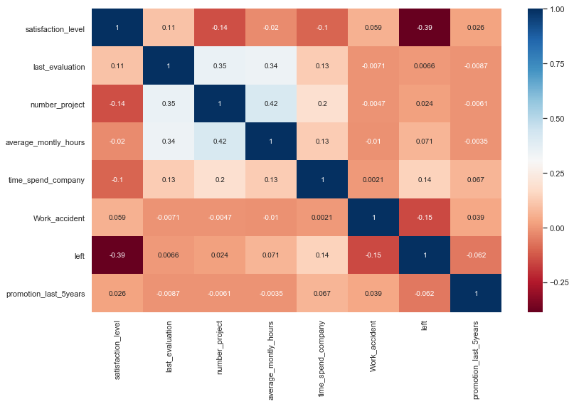
Correlation Analysis
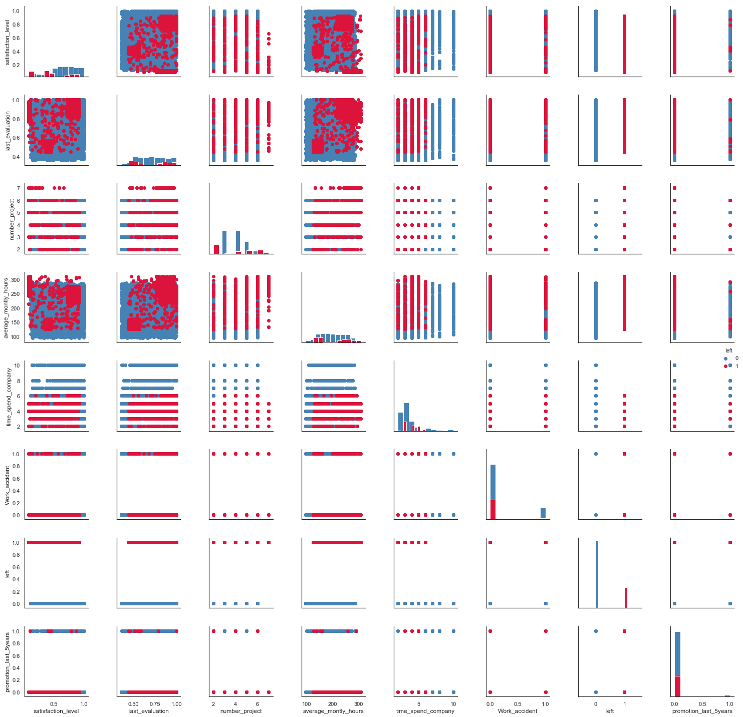
A correlation analysis will allow to identify relationships between the dataset variables. A plot of their distributions highlighting the value of the target variable might also reveal some patterns.
# Correlation Matrix
plt.figure(figsize=(12,8))
sns.heatmap(hr.corr(), cmap='RdBu', annot=True)
plt.tight_layout()
# Pair Plot
plot = sns.PairGrid(hr, hue='left', palette=('steelblue', 'crimson'))
plot = plot.map_diag(plt.hist)
plot = plot.map_offdiag(plt.scatter)
plot.add_legend()
plt.tight_layout()
No strong correlation appears in the dataset. However:
number_projectandaverage_monthly_hourshave a moderate positive correlation (0.42).leftandsatisfaction_levelhave a moderate negative correlation (-0.39).last_evaluationandnumber_projecthave a moderate positive correlation (0.35).last_evaluationandaverage_monthly_hourshave a moderate positive correlation (0.34).
Turnover by Salary Levels
# Salary Levels proportions and turnover rates
print('Salary Levels proportions')
print(hr['salary'].value_counts()/len(hr)*100)
print('\n')
print('Turnover Rate by Salary level')
print(hr.groupby('salary')['left'].mean())
Salary Levels proportions
low       48.776585
medium    42.976198
high       8.247216
Name: salary, dtype: float64

Turnover Rate by Salary level
salary
high      0.066289
low       0.296884
medium    0.204313
Name: left, dtype: float64
The salary level seems to have a great impact on the employee turnover, as higher salaries tend to stay in the company (7% of turnover), whereas lower salaries tend to leave the company (30% of turnover).
Turnover by Departments
# Departments proportions
hr['department'].value_counts()/len(hr)*100
sales          27.601840
technical      18.134542
support        14.860991
IT              8.180545
product_mng     6.013734
marketing       5.720381
RandD           5.247016
accounting      5.113674
hr              4.926995
management      4.200280
Name: department, dtype: float64
# Turnover Rate by Department
hr.groupby('department')['left'].mean().sort_values(ascending=False).plot(kind='bar', color='steelblue')
plt.title('Departure Ratio by Department')
plt.xlabel('')
plt.tight_layout()
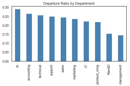
Some observations can be inferred:
- Departure rate differs depending on the department, but no clear outlier is detected.
- HR has the highest turnover rate.
- R&D and Management have a significantly lower turnover rate.
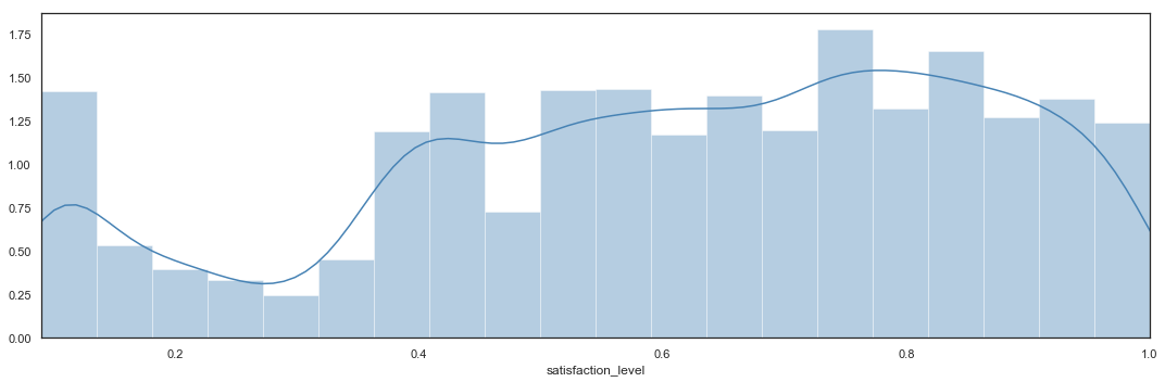
Turnover by Satisfaction Level
# Bar Plot
plt.figure(figsize=(15,5))
sns.distplot(hr.satisfaction_level,
             bins = 20,
             color = 'steelblue').axes.set_xlim(min(hr.satisfaction_level),max(hr.satisfaction_level))
plt.tight_layout()
# Bar Plot with left values
plt.figure(figsize=(15,5))
sns.countplot(hr['satisfaction_level'],
              hue = hr['left'],
              palette = ('steelblue', 'crimson'))
plt.tight_layout()
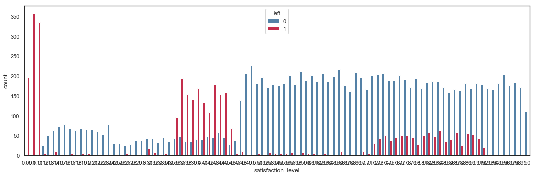
The Satisfaction Level shows 3 interesting areas:
- Employees leave the company below 0.12.
- There is a high rate of departure between 0.36 and 0.46.
- Turnover rate is higher between 0.72 and 0.92.
Employees with very low satisfaction level obviously leave the company. The risky zone is when employees rates their satisfaction just below 0.5. Employees also tend to leave the company when they become moderately satisfied.
Turnover by Last Evaluation
# Bar Plot
plt.figure(figsize=(15,5))
sns.distplot(hr.last_evaluation,
             bins = 20,
             color = 'steelblue').axes.set_xlim(min(hr.last_evaluation),max(hr.last_evaluation))
plt.tight_layout()

# Bar Plot with left values
plt.figure(figsize=(15,5))
sns.countplot(hr['last_evaluation'],
              hue = hr['left'],
              palette = ('steelblue', 'crimson'))
plt.tight_layout()

The Last Evaluation shows 2 interesting areas:
- Turnover rate is higher between 0.45 and 0.57.
- Turnover rate is higher above 0.77.
Employees with low evaluation scores tend to leave the company. A large number of good employees leave the company, maybe to get a better opportunity. Interestingly, the ones with very low scores seem to stay.
Turnover by Number of Projects
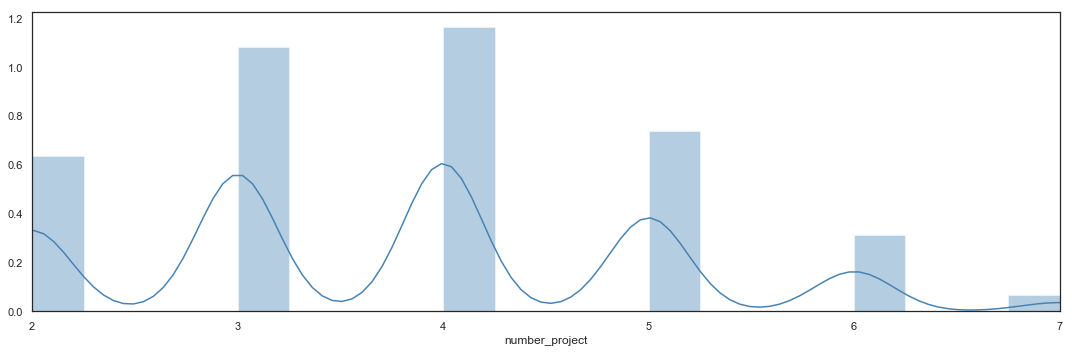
# Bar Plot
plt.figure(figsize=(15,5))
sns.distplot(hr.number_project,
             bins = 20,
             color = 'steelblue').axes.set_xlim(min(hr.number_project),max(hr.number_project))
plt.tight_layout()
# Bar Plot with left values
plt.figure(figsize=(15,5))
sns.countplot(hr['number_project'],
              hue = hr['left'],
              palette = ('steelblue', 'crimson'))
plt.tight_layout()
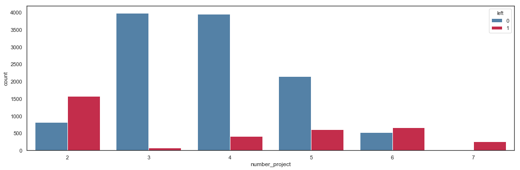
The main observation regarding the number of projects is that employees with only 2 or more than 5 projects have a higher probability to leave the company.
Turnover by Average Monthly Hours
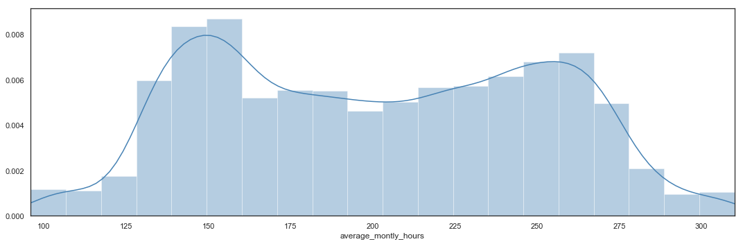
# Bar Plot
plt.figure(figsize=(15,5))
sns.distplot(hr.average_montly_hours,
             bins = 20,
             color = 'steelblue').axes.set_xlim(min(hr.average_montly_hours),max(hr.average_montly_hours))
plt.tight_layout()
# Bar Plot with left values
plt.figure(figsize=(15,5))
sns.countplot(hr['average_montly_hours'],
              hue = hr['left'],
              palette = ('steelblue', 'crimson'))
plt.tight_layout()
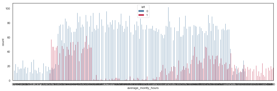
The Average Monthly Hours shows 5 interesting areas:
- Turnover rate is 0% below 125 hours.
- Turnover rate is high between 126 and 161 hours.
- Turnover rate is moderate between 217 and 274 hours.
- Turnover rate is roughly around 50% between 275 and 287 hours.
- Turnover rate is 100% above 288 hours.
Employees with really low numbers of hours per month (below 125) tend to stay in the company, whereas employees working too many hours (above 275 hours) have a high probability to leave the company. A ‘safe’ range is between 161 and 217 hours, which seems to be ideal to keep employees in the company.
Turnover by Time Spent in the Company
# Bar Plot with left values
plt.figure(figsize=(15,5))
sns.countplot(hr['time_spend_company'],
              hue = hr['left'],
              palette = ('steelblue', 'crimson'))
plt.tight_layout()
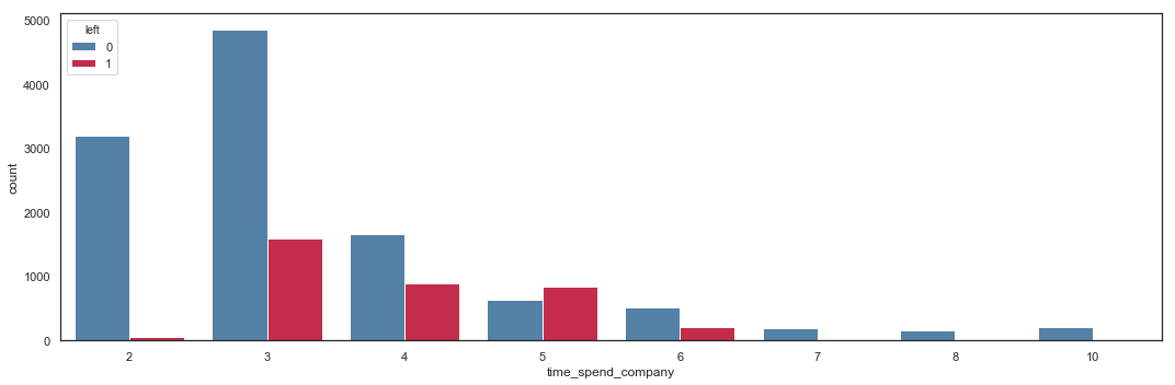
It seems that employees with 3-6 years of services are leaving the company.
Turnover by Work Accident
# Bar Plot with left values
plt.figure(figsize=(15,5))
sns.countplot(hr['Work_accident'],
              hue = hr['left'],
              palette = ('steelblue', 'crimson'))
plt.tight_layout()

Employees with a work accident tend to stay in the company.
Turnover by Promotion within the past 5 years
# Bar Plot with left values
plt.figure(figsize=(15,5))
sns.countplot(hr['promotion_last_5years'],
              hue = hr['left'],
              palette = ('steelblue', 'crimson'))
plt.tight_layout()

print('Turnover Rate if Promotion:', round(len(hr[(hr['promotion_last_5years']==1)&(hr['left']==1)])/len(hr[(hr['promotion_last_5years']==1)])*100,2),'%')
print('Turnover Rate if No Promotion:', round(len(hr[(hr['promotion_last_5years']==0)&(hr['left']==1)])/len(hr[(hr['promotion_last_5years']==0)])*100,2),'%')
Turnover Rate if Promotion: 5.96 %
Turnover Rate if No Promotion: 24.2 %
It appears that employees with a promotion within the past 5 years have less propensity to leave the company.
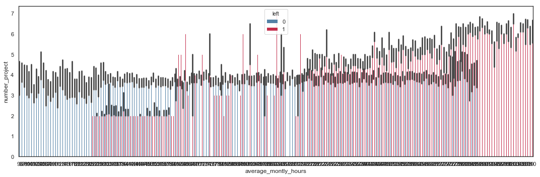
Number of Projects vs Average Monthly Hours
# Bar Plot with left values
plt.figure(figsize=(15,5))
sns.barplot(x=hr.average_montly_hours,
            y=hr.number_project,
            hue=hr.left,
            palette = ('steelblue', 'crimson'))
plt.tight_layout()
# Scatter Plot with left values
plt.figure(figsize=(15,5))
sns.scatterplot(x=hr.average_montly_hours,
            y=hr.number_project,
            hue=hr.left,
            palette = ('steelblue', 'crimson'))
plt.tight_layout()
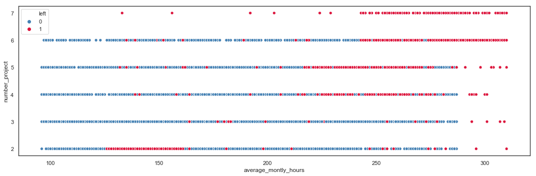
It appears that:
- employees with more than 4 projects and working more than 217 hours tend to leave the company.
- employees with less than 3 projects and working less than 161 hours tend to leave the company.
A high or a low workload seem to push employees out.
Number of Projects vs Last Evaluation
# Bar Plot with left values
plt.figure(figsize=(15,5))
sns.barplot(x=hr.last_evaluation,
            y=hr.number_project,
            hue=hr.left,
            palette = ('steelblue', 'crimson'))
plt.tight_layout()

# Scatter Plot with left values
plt.figure(figsize=(15,5))
sns.scatterplot(x=hr.last_evaluation,
            y=hr.number_project,
            hue=hr.left,
            palette = ('steelblue', 'crimson'))
plt.tight_layout()
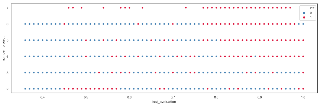
Employees with more than 4 projects seem to have higher evaluations but leave the company. Employees with 2 projects and a low evaluation leave the company.
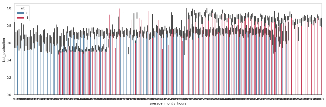
Last Evaluation vs Average Monthly Hours
# Bar Plot with left values
plt.figure(figsize=(15,5))
sns.barplot(x=hr.average_montly_hours,
            y=hr.last_evaluation,
            hue=hr.left,
            palette = ('steelblue', 'crimson'))
plt.tight_layout()
# Scatter Plot with left values
plt.figure(figsize=(15,5))
sns.scatterplot(x=hr.average_montly_hours,
            y=hr.last_evaluation,
            hue=hr.left,
            palette = ('steelblue', 'crimson'))
plt.tight_layout()

Employees with high evaluation and working more than 217 hours tend to leave the company. Employees with evaluation around 0.5 and working between 125 and 161 hours tend to leave the company.
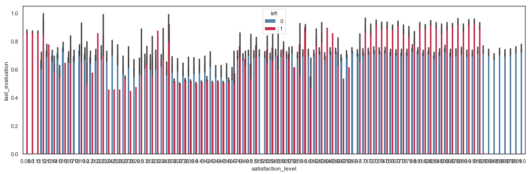
Last Evaluation vs Satisfaction Level
# Bar Plot with left values
plt.figure(figsize=(15,5))
sns.barplot(x=hr.satisfaction_level,
            y=hr.last_evaluation,
            hue=hr.left,
            palette = ('steelblue', 'crimson'))
plt.tight_layout()
# Scatter Plot with left values
plt.figure(figsize=(15,5))
sns.scatterplot(x=hr.satisfaction_level,
            y=hr.last_evaluation,
            hue=hr.left,
            palette = ('steelblue', 'crimson'))
plt.tight_layout()

Employees with satisfaction level below 0.11 tend to leave the company. Employees with satisfaction level between 0.35 and 0.46 and with last evaluation between 0.44 and 0.57 tend to leave the company. Employees with satisfaction level between 0.71 and 0.92 and with last evaluation between 0.76 and 1 tend to leave the company.
Encoding Categorical Variables
The variable salary will be encoded using ordinal encoding and department will be encoded using one-hot encoding.
# Encoding the variable salary
salary_dict = {'low':0,'medium':1,'high':2}
hr['salary_num'] = hr.salary.map(salary_dict)
hr.drop('salary', inplace=True, axis=1)
hr = hr.rename(index=str, columns={'salary_num':'salary'})
hr.head()
| satisfaction_level | last_evaluation | number_project | average_montly_hours | time_spend_company | Work_accident | left | promotion_last_5years | department | salary | |
|---|---|---|---|---|---|---|---|---|---|---|
| 0 | 0.38 | 0.53 | 2 | 157 | 3 | 0 | 1 | 0 | sales | 0 |
| 1 | 0.80 | 0.86 | 5 | 262 | 6 | 0 | 1 | 0 | sales | 1 |
| 2 | 0.11 | 0.88 | 7 | 272 | 4 | 0 | 1 | 0 | sales | 1 |
| 3 | 0.72 | 0.87 | 5 | 223 | 5 | 0 | 1 | 0 | sales | 0 |
| 4 | 0.37 | 0.52 | 2 | 159 | 3 | 0 | 1 | 0 | sales | 0 |
def numerical_features(df):
    columns = df.columns
    return df._get_numeric_data().columns

def categorical_features(df):
    numerical_columns = numerical_features(df)
    return(list(set(df.columns) - set(numerical_columns)))

def onehot_encode(df):
    numericals = df.get(numerical_features(df))
    new_df = numericals.copy()
    for categorical_column in categorical_features(df):
        new_df = pd.concat([new_df,
                            pd.get_dummies(df[categorical_column],
                                           prefix=categorical_column)],
                           axis=1)
    return new_df
hr_encoded = onehot_encode(hr)
hr_encoded.head()
| satisfaction_level | last_evaluation | number_project | average_montly_hours | time_spend_company | Work_accident | left | promotion_last_5years | salary | department_IT | department_RandD | department_accounting | department_hr | department_management | department_marketing | department_product_mng | department_sales | department_support | department_technical | |
|---|---|---|---|---|---|---|---|---|---|---|---|---|---|---|---|---|---|---|---|
| 0 | 0.38 | 0.53 | 2 | 157 | 3 | 0 | 1 | 0 | 0 | 0 | 0 | 0 | 0 | 0 | 0 | 0 | 1 | 0 | 0 |
| 1 | 0.80 | 0.86 | 5 | 262 | 6 | 0 | 1 | 0 | 1 | 0 | 0 | 0 | 0 | 0 | 0 | 0 | 1 | 0 | 0 |
| 2 | 0.11 | 0.88 | 7 | 272 | 4 | 0 | 1 | 0 | 1 | 0 | 0 | 0 | 0 | 0 | 0 | 0 | 1 | 0 | 0 |
| 3 | 0.72 | 0.87 | 5 | 223 | 5 | 0 | 1 | 0 | 0 | 0 | 0 | 0 | 0 | 0 | 0 | 0 | 1 | 0 | 0 |
| 4 | 0.37 | 0.52 | 2 | 159 | 3 | 0 | 1 | 0 | 0 | 0 | 0 | 0 | 0 | 0 | 0 | 0 | 1 | 0 | 0 |
df_desc(hr_encoded)
| dtype | NAs | Numerical | Boolean | Categorical | |
|---|---|---|---|---|---|
| satisfaction_level | float64 | 0 | True | False | False |
| last_evaluation | float64 | 0 | True | False | False |
| number_project | int64 | 0 | True | False | False |
| average_montly_hours | int64 | 0 | True | False | False |
| time_spend_company | int64 | 0 | True | False | False |
| Work_accident | int64 | 0 | False | True | False |
| left | int64 | 0 | False | True | False |
| promotion_last_5years | int64 | 0 | False | True | False |
| salary | int64 | 0 | True | False | False |
| department_IT | uint8 | 0 | False | True | False |
| department_RandD | uint8 | 0 | False | True | False |
| department_accounting | uint8 | 0 | False | True | False |
| department_hr | uint8 | 0 | False | True | False |
| department_management | uint8 | 0 | False | True | False |
| department_marketing | uint8 | 0 | False | True | False |
| department_product_mng | uint8 | 0 | False | True | False |
| department_sales | uint8 | 0 | False | True | False |
| department_support | uint8 | 0 | False | True | False |
| department_technical | uint8 | 0 | False | True | False |
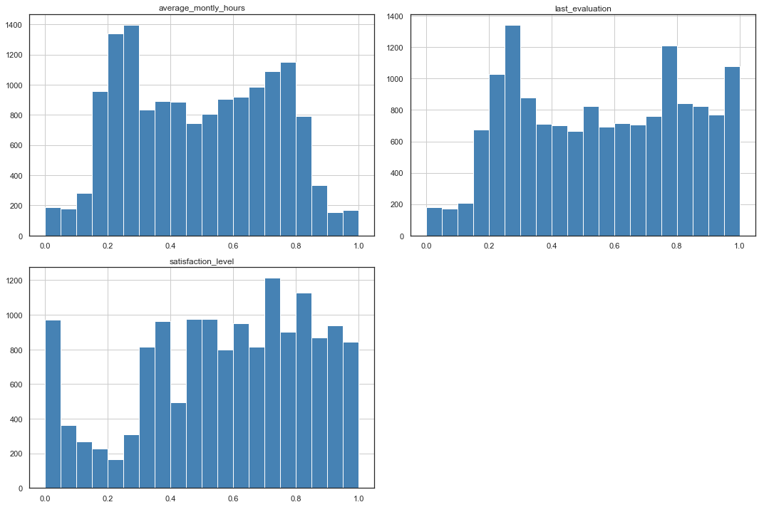
Scaling and Skewness
Numerical variables average_monthly_hours, last_evaluation and satisfaction_level are scaled to remove any influence of their difference in value ranges on the model.
hr_encoded[['satisfaction_level',
           'last_evaluation',
           'average_montly_hours'
           ]].hist(bins = 20, figsize = (15,10), color = 'steelblue')
plt.tight_layout()

hr_encoded[['satisfaction_level',
           'last_evaluation',
           'average_montly_hours'
           ]].describe()
| satisfaction_level | last_evaluation | average_montly_hours | |
|---|---|---|---|
| count | 14999.000000 | 14999.000000 | 14999.000000 |
| mean | 0.612834 | 0.716102 | 201.050337 |
| std | 0.248631 | 0.171169 | 49.943099 |
| min | 0.090000 | 0.360000 | 96.000000 |
| 25% | 0.440000 | 0.560000 | 156.000000 |
| 50% | 0.640000 | 0.720000 | 200.000000 |
| 75% | 0.820000 | 0.870000 | 245.000000 |
| max | 1.000000 | 1.000000 | 310.000000 |
scaler = preprocessing.MinMaxScaler()
hr_scaled_part = scaler.fit_transform(hr_encoded[['satisfaction_level',
                                                  'last_evaluation',
                                                  'average_montly_hours']])
hr_scaled_part = pd.DataFrame(hr_scaled_part, columns=list(['satisfaction_level',
                                                  'last_evaluation',
                                                  'average_montly_hours']))
hr_scaled_part[['satisfaction_level',
                'last_evaluation',
                'average_montly_hours']].hist(bins = 20, figsize = (15,10), color = 'steelblue')
plt.tight_layout()

hr_scaled_part.describe()
| satisfaction_level | last_evaluation | average_montly_hours | |
|---|---|---|---|
| count | 14999.000000 | 14999.000000 | 14999.000000 |
| mean | 0.574542 | 0.556409 | 0.490889 |
| std | 0.273220 | 0.267452 | 0.233379 |
| min | 0.000000 | 0.000000 | 0.000000 |
| 25% | 0.384615 | 0.312500 | 0.280374 |
| 50% | 0.604396 | 0.562500 | 0.485981 |
| 75% | 0.802198 | 0.796875 | 0.696262 |
| max | 1.000000 | 1.000000 | 1.000000 |
The skewness of the scaled variables is then fixed.
def feature_skewness(df):
    numeric_dtypes = ['int16', 'int32', 'int64',
                      'float16', 'float32', 'float64']
    numeric_features = []
    for i in df.columns:
        if df[i].dtype in numeric_dtypes:
            numeric_features.append(i)

    feature_skew = df[numeric_features].apply(
        lambda x: skew(x)).sort_values(ascending=False)
    skews = pd.DataFrame({'skew':feature_skew})
    return feature_skew, numeric_features
def fix_skewness(df):
    feature_skew, numeric_features = feature_skewness(df)
    high_skew = feature_skew[feature_skew > 0.5]
    skew_index = high_skew.index

    for i in skew_index:
        df[i] = boxcox1p(df[i], boxcox_normmax(df[i]+1))

    skew_features = df[numeric_features].apply(
        lambda x: skew(x)).sort_values(ascending=False)
    skews = pd.DataFrame({'skew':skew_features})
    return df
hr_skewed_part = fix_skewness(hr_scaled_part)
hr_skewed_part.hist(bins = 20, figsize = (15,10), color = 'steelblue')
plt.tight_layout()
hr_skewed_part.describe()
| satisfaction_level | last_evaluation | average_montly_hours | |
|---|---|---|---|
| count | 14999.000000 | 14999.000000 | 14999.000000 |
| mean | 0.574542 | 0.556409 | 0.490889 |
| std | 0.273220 | 0.267452 | 0.233379 |
| min | 0.000000 | 0.000000 | 0.000000 |
| 25% | 0.384615 | 0.312500 | 0.280374 |
| 50% | 0.604396 | 0.562500 | 0.485981 |
| 75% | 0.802198 | 0.796875 | 0.696262 |
| max | 1.000000 | 1.000000 | 1.000000 |
The resulting values aren’t different than the initial ones, showing that the data wasn’t skewed.
hr_simple = hr_encoded.copy()
hr_simple.drop(['satisfaction_level',
                'last_evaluation',
                'average_montly_hours'], inplace=True, axis=1)

hr_ready = pd.DataFrame()
hr_simple.reset_index(drop=True, inplace=True)
hr_skewed_part.reset_index(drop=True, inplace=True)

hr_ready = pd.concat([hr_skewed_part,hr_simple], axis=1, sort=False, ignore_index=False)

# hr_ready['number_project'] = hr_ready['number_project'].astype('category').cat.codes
# hr_ready['time_spend_company'] = hr_ready['time_spend_company'].astype('category').cat.codes

hr_ready.head()
| satisfaction_level | last_evaluation | average_montly_hours | number_project | time_spend_company | Work_accident | left | promotion_last_5years | salary | department_IT | department_RandD | department_accounting | department_hr | department_management | department_marketing | department_product_mng | department_sales | department_support | department_technical | |
|---|---|---|---|---|---|---|---|---|---|---|---|---|---|---|---|---|---|---|---|
| 0 | 0.318681 | 0.265625 | 0.285047 | 2 | 3 | 0 | 1 | 0 | 0 | 0 | 0 | 0 | 0 | 0 | 0 | 0 | 1 | 0 | 0 |
| 1 | 0.780220 | 0.781250 | 0.775701 | 5 | 6 | 0 | 1 | 0 | 1 | 0 | 0 | 0 | 0 | 0 | 0 | 0 | 1 | 0 | 0 |
| 2 | 0.021978 | 0.812500 | 0.822430 | 7 | 4 | 0 | 1 | 0 | 1 | 0 | 0 | 0 | 0 | 0 | 0 | 0 | 1 | 0 | 0 |
| 3 | 0.692308 | 0.796875 | 0.593458 | 5 | 5 | 0 | 1 | 0 | 0 | 0 | 0 | 0 | 0 | 0 | 0 | 0 | 1 | 0 | 0 |
| 4 | 0.307692 | 0.250000 | 0.294393 | 2 | 3 | 0 | 1 | 0 | 0 | 0 | 0 | 0 | 0 | 0 | 0 | 0 | 1 | 0 | 0 |
df_desc(hr_ready)
| dtype | NAs | Numerical | Boolean | Categorical | |
|---|---|---|---|---|---|
| satisfaction_level | float64 | 0 | True | False | False |
| last_evaluation | float64 | 0 | True | False | False |
| average_montly_hours | float64 | 0 | True | False | False |
| number_project | int64 | 0 | True | False | False |
| time_spend_company | int64 | 0 | True | False | False |
| Work_accident | int64 | 0 | False | True | False |
| left | int64 | 0 | False | True | False |
| promotion_last_5years | int64 | 0 | False | True | False |
| salary | int64 | 0 | True | False | False |
| department_IT | uint8 | 0 | False | True | False |
| department_RandD | uint8 | 0 | False | True | False |
| department_accounting | uint8 | 0 | False | True | False |
| department_hr | uint8 | 0 | False | True | False |
| department_management | uint8 | 0 | False | True | False |
| department_marketing | uint8 | 0 | False | True | False |
| department_product_mng | uint8 | 0 | False | True | False |
| department_sales | uint8 | 0 | False | True | False |
| department_support | uint8 | 0 | False | True | False |
| department_technical | uint8 | 0 | False | True | False |
hr_ready.describe()
| satisfaction_level | last_evaluation | average_montly_hours | number_project | time_spend_company | Work_accident | left | promotion_last_5years | salary | department_IT | department_RandD | department_accounting | department_hr | department_management | department_marketing | department_product_mng | department_sales | department_support | department_technical | |
|---|---|---|---|---|---|---|---|---|---|---|---|---|---|---|---|---|---|---|---|
| count | 14999.000000 | 14999.000000 | 14999.000000 | 14999.000000 | 14999.000000 | 14999.000000 | 14999.000000 | 14999.000000 | 14999.000000 | 14999.000000 | 14999.000000 | 14999.000000 | 14999.000000 | 14999.000000 | 14999.000000 | 14999.000000 | 14999.000000 | 14999.000000 | 14999.000000 |
| mean | 0.574542 | 0.556409 | 0.490889 | 3.803054 | 3.498233 | 0.144610 | 0.238083 | 0.021268 | 0.594706 | 0.081805 | 0.052470 | 0.051137 | 0.049270 | 0.042003 | 0.057204 | 0.060137 | 0.276018 | 0.148610 | 0.181345 |
| std | 0.273220 | 0.267452 | 0.233379 | 1.232592 | 1.460136 | 0.351719 | 0.425924 | 0.144281 | 0.637183 | 0.274077 | 0.222981 | 0.220284 | 0.216438 | 0.200602 | 0.232239 | 0.237749 | 0.447041 | 0.355715 | 0.385317 |
| min | 0.000000 | 0.000000 | 0.000000 | 2.000000 | 2.000000 | 0.000000 | 0.000000 | 0.000000 | 0.000000 | 0.000000 | 0.000000 | 0.000000 | 0.000000 | 0.000000 | 0.000000 | 0.000000 | 0.000000 | 0.000000 | 0.000000 |
| 25% | 0.384615 | 0.312500 | 0.280374 | 3.000000 | 3.000000 | 0.000000 | 0.000000 | 0.000000 | 0.000000 | 0.000000 | 0.000000 | 0.000000 | 0.000000 | 0.000000 | 0.000000 | 0.000000 | 0.000000 | 0.000000 | 0.000000 |
| 50% | 0.604396 | 0.562500 | 0.485981 | 4.000000 | 3.000000 | 0.000000 | 0.000000 | 0.000000 | 1.000000 | 0.000000 | 0.000000 | 0.000000 | 0.000000 | 0.000000 | 0.000000 | 0.000000 | 0.000000 | 0.000000 | 0.000000 |
| 75% | 0.802198 | 0.796875 | 0.696262 | 5.000000 | 4.000000 | 0.000000 | 0.000000 | 0.000000 | 1.000000 | 0.000000 | 0.000000 | 0.000000 | 0.000000 | 0.000000 | 0.000000 | 0.000000 | 1.000000 | 0.000000 | 0.000000 |
| max | 1.000000 | 1.000000 | 1.000000 | 7.000000 | 10.000000 | 1.000000 | 1.000000 | 1.000000 | 2.000000 | 1.000000 | 1.000000 | 1.000000 | 1.000000 | 1.000000 | 1.000000 | 1.000000 | 1.000000 | 1.000000 | 1.000000 |
hr_ready.hist(bins = 20, figsize = (15,10), color = 'steelblue')
plt.tight_layout()
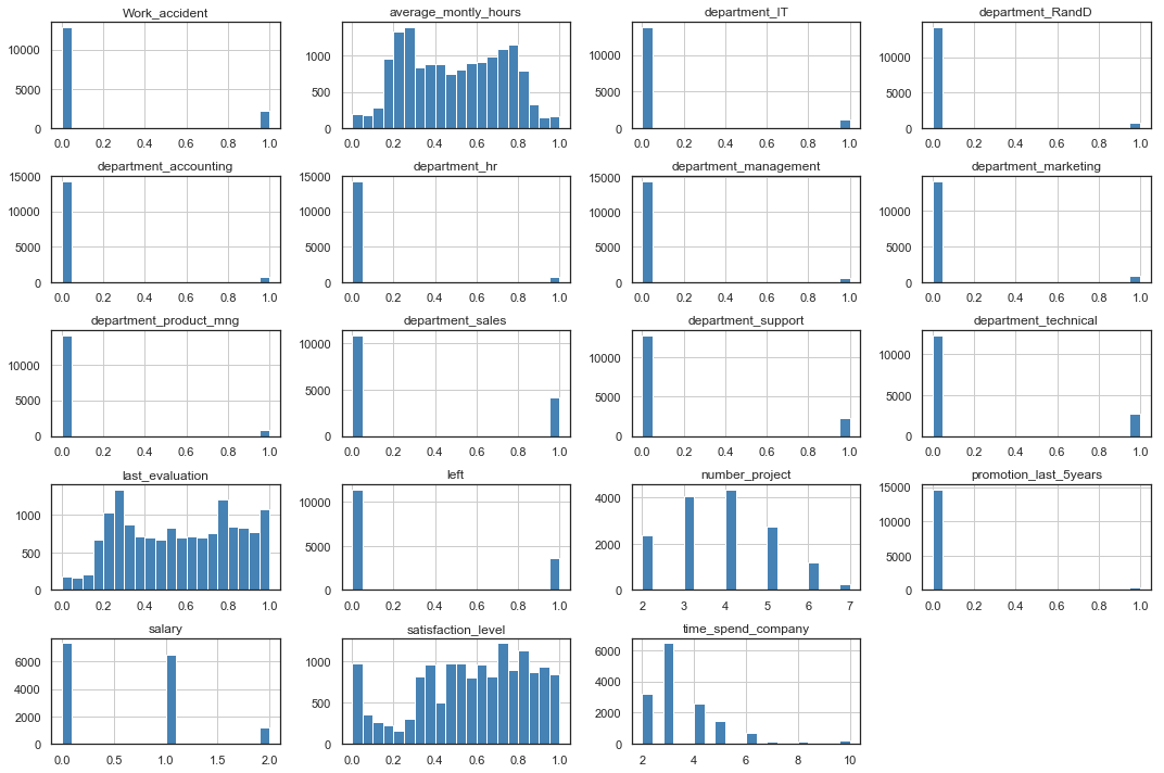
The dataset is now ready to go through the baseline and feature engineering phases.
Training/Test Split
The model target left is defined, taking all other variables as features. The dataset is split in a train set and a test set, using a random split with ratio 70|30.
target = 'left'

split_ratio = 0.3
seed = 806

def split_dataset(df, target, split_ratio=0.3, seed=806):
    features = list(df)
    features.remove(target)

    X = df[features]
    y = df[[target]]

    X_train, X_test, y_train, y_test = train_test_split(X, y, test_size=split_ratio, random_state=seed)

    return X, y, X_train, X_test, y_train, y_test

X, y, X_train, X_test, y_train, y_test = split_dataset(hr_ready, target, split_ratio, seed)

print('Features:',X.shape[0], 'items | ', X.shape[1],'columns')
print('Target:',y.shape[0], 'items | ', y.shape[1],'columns')
print('Features Train:',X_train.shape[0], 'items | ', X_train.shape[1],'columns')
print('Features Test:',X_test.shape[0], 'items | ', X_test.shape[1],'columns')
print('Target Train:',y_train.shape[0], 'items | ', y_train.shape[1],'columns')
print('Target Test:',y_test.shape[0], 'items | ', y_test.shape[1],'columns')
Features: 14999 items |  18 columns
Target: 14999 items |  1 columns
Features Train: 10499 items |  18 columns
Features Test: 4500 items |  18 columns
Target Train: 10499 items |  1 columns
Target Test: 4500 items |  1 columns
Baseline
A logistic regression algorithm will be used to develop this classification model.
lr = LogisticRegression(solver='lbfgs', max_iter = 300)
def lr_run(model, X_train, y_train, X_test, y_test):
    result = model.fit(X_train, y_train.values.ravel())

    y_pred = model.predict(X_test)
    acc_test = model.score(X_test, y_test)
    coefficients = pd.concat([pd.DataFrame(X_train.columns, columns=['Feature']), pd.DataFrame(np.transpose(model.coef_), columns=['Coef.'])], axis = 1)
    coefficients.loc[-1] = ['intercept.', model.intercept_[0]]
    coefficients.index = coefficients.index + 1
    coefficients = coefficients.sort_index()

    print('Accuracy on test: {:.3f}'.format(acc_test))
    print()
    print(classification_report(y_test, y_pred))
    print('Confusion Matrix:')
    print(confusion_matrix(y_test, y_pred))
    print()
    print(coefficients)
lr_run(lr, X_train, y_train, X_test, y_test)
Accuracy on test: 0.797

              precision    recall  f1-score   support

           0       0.82      0.94      0.88      3435
           1       0.63      0.34      0.44      1065

   micro avg       0.80      0.80      0.80      4500
   macro avg       0.73      0.64      0.66      4500
weighted avg       0.78      0.80      0.77      4500

Confusion Matrix:
[[3220  215]
 [ 700  365]]

                   Feature     Coef.
0               intercept.  0.652320
1       satisfaction_level -3.616897
2          last_evaluation  0.440219
3     average_montly_hours  0.910047
4           number_project -0.285360
5       time_spend_company  0.245415
6            Work_accident -1.394756
7    promotion_last_5years -1.189347
8                   salary -0.695794
9            department_IT -0.065202
10        department_RandD -0.474089
11   department_accounting  0.069995
12           department_hr  0.336695
13   department_management -0.352861
14    department_marketing  0.062124
15  department_product_mng  0.040313
16        department_sales  0.019114
17      department_support  0.230860
18    department_technical  0.147269
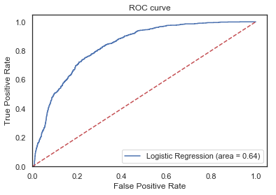
The ROC Curve can be plot for the model.
def plot_roc(model, X_test, y_test):
    logit_roc_auc = roc_auc_score(y_test, model.predict(X_test))
    fpr, tpr, thresholds = roc_curve(y_test, model.predict_proba(X_test)[:,1])
    plt.figure()
    plt.plot(fpr, tpr, label='Logistic Regression (area = %0.2f)' % logit_roc_auc)
    plt.plot([0, 1], [0, 1], 'r--')
    plt.xlim([0.0, 1.05])
    plt.ylim([0.0, 1.05])
    plt.xlabel('False Positive Rate')
    plt.ylabel('True Positive Rate')
    plt.title('ROC curve')
    plt.legend(loc="lower right")
    plt.show();
plot_roc(lr, X_test, y_test)
Feature Engineering
Cross Validation Strategy
The model is cross-validated using a 10-fold cross validation and returning the average accuracy.
Example based on the baseline:
def cv_acc (model, X_train, y_train, n_splits, seed):
    kfold = model_selection.KFold(n_splits=n_splits, random_state=seed)
    scoring = 'accuracy'
    results = model_selection.cross_val_score(model, X_train, y_train.values.ravel(), cv=kfold, scoring=scoring)
    print("10-fold cross validation average accuracy: %.3f" % (results.mean()))
    print()
    for i in range(len(results)):
        print('Iteration', '{:>2}'.format(i+1), '| Accuracy: {:.2f}'.format(results[i]))
cv_acc(lr, X_train, y_train, 10, seed)
10-fold cross validation average accuracy: 0.789

Iteration  1 | Accuracy: 0.79
Iteration  2 | Accuracy: 0.77
Iteration  3 | Accuracy: 0.78
Iteration  4 | Accuracy: 0.80
Iteration  5 | Accuracy: 0.81
Iteration  6 | Accuracy: 0.79
Iteration  7 | Accuracy: 0.79
Iteration  8 | Accuracy: 0.80
Iteration  9 | Accuracy: 0.79
Iteration 10 | Accuracy: 0.77
Features Construction
The dataset is copied to add or modify features.
hr_fe = hr_ready.copy()
Bin Satisfaction Level
Based on the EDA, we can bin the Satisfaction Level into 6 bins.
bins = [-1, 0.03, 0.29, 0.41, 0.69, 0.92, 1]
labels=['(0.00, 0.11]','(0.11, 0.35]','(0.35, 0.46]','(0.46, 0.71]','(0.71, 0.92]','(0.92, 1.00]']
hr_fe['satisfaction_level_bin'] = pd.cut(hr_fe.satisfaction_level, bins, labels=labels)
hr_fe.satisfaction_level_bin.value_counts()
(0.71, 0.92]    4765
(0.46, 0.71]    4689
(0.35, 0.46]    2012
(0.92, 1.00]    1362
(0.11, 0.35]    1283
(0.00, 0.11]     888
Name: satisfaction_level_bin, dtype: int64
plt.figure(figsize=(15,5))
sns.countplot(x=hr_fe.satisfaction_level,
              hue=hr_fe.satisfaction_level_bin,
              palette = sns.color_palette("hls", 6),
              dodge = False)
plt.tight_layout()

hr_fe_1 = hr_fe.copy()
hr_fe_1 = onehot_encode(hr_fe_1)
hr_fe_1.drop('satisfaction_level', inplace=True, axis=1)
X_fe_1, y_fe_1, X_fe_1_train, X_fe_1_test, y_fe_1_train, y_fe_1_test = split_dataset(hr_fe_1, target, split_ratio, seed)
cv_acc(lr, X_fe_1_train, y_fe_1_train, 10, seed)
print()
lr_run(lr, X_fe_1_train, y_fe_1_train, X_fe_1_test, y_fe_1_test)
10-fold cross validation average accuracy: 0.916

Iteration  1 | Accuracy: 0.92
Iteration  2 | Accuracy: 0.92
Iteration  3 | Accuracy: 0.90
Iteration  4 | Accuracy: 0.91
Iteration  5 | Accuracy: 0.93
Iteration  6 | Accuracy: 0.92
Iteration  7 | Accuracy: 0.92
Iteration  8 | Accuracy: 0.92
Iteration  9 | Accuracy: 0.91
Iteration 10 | Accuracy: 0.91

Accuracy on test: 0.914

              precision    recall  f1-score   support

           0       0.94      0.95      0.94      3435
           1       0.83      0.79      0.81      1065

   micro avg       0.91      0.91      0.91      4500
   macro avg       0.89      0.87      0.88      4500
weighted avg       0.91      0.91      0.91      4500

Confusion Matrix:
[[3266  169]
 [ 220  845]]

                                Feature     Coef.
0                            intercept. -4.095534
1                       last_evaluation  1.885761
2                  average_montly_hours  1.871660
3                        number_project -0.118954
4                    time_spend_company  0.433360
5                         Work_accident -1.199810
6                 promotion_last_5years -1.053322
7                                salary -0.727225
8                         department_IT -0.042518
9                      department_RandD -0.274695
10                department_accounting  0.042351
11                        department_hr  0.587357
12                department_management -0.686777
13                 department_marketing  0.032783
14               department_product_mng -0.083776
15                     department_sales -0.012227
16                   department_support  0.255890
17                 department_technical  0.198702
18  satisfaction_level_bin_(0.00, 0.11]  5.196334
19  satisfaction_level_bin_(0.11, 0.35] -1.585870
20  satisfaction_level_bin_(0.35, 0.46]  3.741138
21  satisfaction_level_bin_(0.46, 0.71] -2.639350
22  satisfaction_level_bin_(0.71, 0.92] -0.409764
23  satisfaction_level_bin_(0.92, 1.00] -4.285400
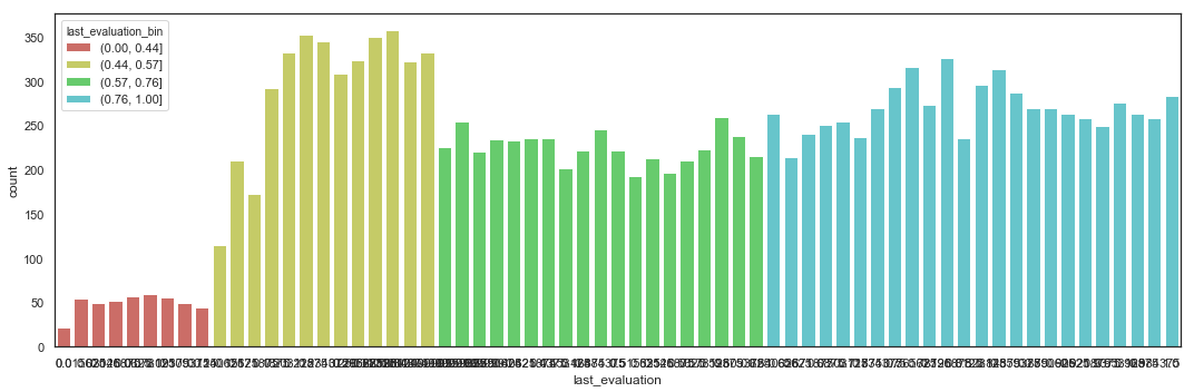
Bin Last Evaluation
Based on the EDA, we can bin the Last Evaluation into 4 bins.
bins = [-1, 0.14, 0.34, 0.64, 1]
labels=['(0.00, 0.44]','(0.44, 0.57]','(0.57, 0.76]','(0.76, 1.00]']
hr_fe['last_evaluation_bin'] = pd.cut(hr_fe.last_evaluation, bins, labels=labels)
hr_fe_1['last_evaluation_bin'] = pd.cut(hr_fe_1.last_evaluation, bins, labels=labels)
hr_fe_1.last_evaluation_bin.value_counts()
(0.76, 1.00]    6458
(0.57, 0.76]    4279
(0.44, 0.57]    3817
(0.00, 0.44]     445
Name: last_evaluation_bin, dtype: int64
plt.figure(figsize=(15,5))
sns.countplot(x=hr_fe_1.last_evaluation,
              hue=hr_fe_1.last_evaluation_bin,
              palette = sns.color_palette("hls", 6),
              dodge = False)
plt.tight_layout()
hr_fe_2 = hr_fe_1.copy()
hr_fe_2 = onehot_encode(hr_fe_2)
hr_fe_2.drop('last_evaluation', inplace=True, axis=1)
X_fe_2, y_fe_2, X_fe_2_train, X_fe_2_test, y_fe_2_train, y_fe_2_test = split_dataset(hr_fe_2, target, split_ratio, seed)
cv_acc(lr, X_fe_2_train, y_fe_2_train, 10, seed)
print()
lr_run(lr, X_fe_2_train, y_fe_2_train, X_fe_2_test, y_fe_2_test)
10-fold cross validation average accuracy: 0.935

Iteration  1 | Accuracy: 0.93
Iteration  2 | Accuracy: 0.93
Iteration  3 | Accuracy: 0.93
Iteration  4 | Accuracy: 0.93
Iteration  5 | Accuracy: 0.94
Iteration  6 | Accuracy: 0.93
Iteration  7 | Accuracy: 0.95
Iteration  8 | Accuracy: 0.94
Iteration  9 | Accuracy: 0.93
Iteration 10 | Accuracy: 0.93

Accuracy on test: 0.936

              precision    recall  f1-score   support

           0       0.95      0.97      0.96      3435
           1       0.88      0.84      0.86      1065

   micro avg       0.94      0.94      0.94      4500
   macro avg       0.92      0.90      0.91      4500
weighted avg       0.94      0.94      0.94      4500

Confusion Matrix:
[[3315  120]
 [ 167  898]]

                                Feature     Coef.
0                            intercept. -5.603085
1                  average_montly_hours  2.193703
2                        number_project  0.058753
3                    time_spend_company  0.462998
4                         Work_accident -1.172361
5                 promotion_last_5years -0.951366
6                                salary -0.723623
7                         department_IT -0.095618
8                      department_RandD -0.213647
9                 department_accounting  0.034969
10                        department_hr  0.620110
11                department_management -0.743974
12                 department_marketing  0.043686
13               department_product_mng -0.108800
14                     department_sales -0.000440
15                   department_support  0.229240
16                 department_technical  0.235322
17  satisfaction_level_bin_(0.00, 0.11]  4.810074
18  satisfaction_level_bin_(0.11, 0.35] -1.521279
19  satisfaction_level_bin_(0.35, 0.46]  3.612606
20  satisfaction_level_bin_(0.46, 0.71] -2.507489
21  satisfaction_level_bin_(0.71, 0.92] -0.262796
22  satisfaction_level_bin_(0.92, 1.00] -4.130269
23     last_evaluation_bin_(0.00, 0.44] -3.358944
24     last_evaluation_bin_(0.44, 0.57]  2.066166
25     last_evaluation_bin_(0.57, 0.76] -0.739115
26     last_evaluation_bin_(0.76, 1.00]  2.032740
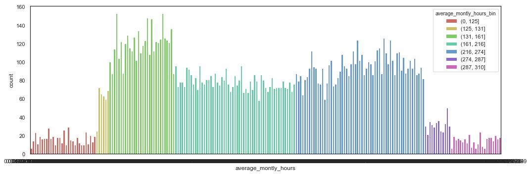
Bin Average Monthly Hours
Based on the EDA, we can bin the Average Monthly Hours into 7 bins.
bins = [-1, 0.14, 0.165, 0.304, 0.565, 0.840, 0.897, 1]
labels=['(0, 125]','(125, 131]','(131, 161]','(161, 216]','(216, 274]','(274, 287]','(287, 310]']
hr_fe['average_montly_hours_bin'] = pd.cut(hr_fe.average_montly_hours, bins, labels=labels)
hr_fe_2['average_montly_hours_bin'] = pd.cut(hr_fe_2.average_montly_hours, bins, labels=labels)
hr_fe_2.average_montly_hours_bin.value_counts()
(216, 274]    5573
(161, 216]    4290
(131, 161]    3588
(0, 125]       486
(274, 287]     379
(125, 131]     353
(287, 310]     330
Name: average_montly_hours_bin, dtype: int64
plt.figure(figsize=(15,5))
sns.countplot(x=hr_fe_2.average_montly_hours,
              hue=hr_fe_2.average_montly_hours_bin,
              palette = sns.color_palette("hls", 7),
              dodge = False)
plt.tight_layout()
hr_fe_3 = hr_fe_2.copy()
hr_fe_3 = onehot_encode(hr_fe_3)
hr_fe_3.drop('average_montly_hours', inplace=True, axis=1)
X_fe_3, y_fe_3, X_fe_3_train, X_fe_3_test, y_fe_3_train, y_fe_3_test = split_dataset(hr_fe_3, target, split_ratio, seed)
cv_acc(lr, X_fe_3_train, y_fe_3_train, 10, seed)
print()
lr_run(lr, X_fe_3_train, y_fe_3_train, X_fe_3_test, y_fe_3_test)
10-fold cross validation average accuracy: 0.944

Iteration  1 | Accuracy: 0.95
Iteration  2 | Accuracy: 0.94
Iteration  3 | Accuracy: 0.94
Iteration  4 | Accuracy: 0.94
Iteration  5 | Accuracy: 0.95
Iteration  6 | Accuracy: 0.94
Iteration  7 | Accuracy: 0.95
Iteration  8 | Accuracy: 0.95
Iteration  9 | Accuracy: 0.94
Iteration 10 | Accuracy: 0.93

Accuracy on test: 0.945

              precision    recall  f1-score   support

           0       0.96      0.97      0.96      3435
           1       0.91      0.86      0.88      1065

   micro avg       0.95      0.95      0.95      4500
   macro avg       0.93      0.92      0.92      4500
weighted avg       0.94      0.95      0.94      4500

Confusion Matrix:
[[3340   95]
 [ 151  914]]

                                Feature     Coef.
0                            intercept. -4.893750
1                        number_project  0.162189
2                    time_spend_company  0.452624
3                         Work_accident -1.155125
4                 promotion_last_5years -0.830508
5                                salary -0.709974
6                         department_IT -0.047511
7                      department_RandD -0.287313
8                 department_accounting  0.011035
9                         department_hr  0.541995
10                department_management -0.624920
11                 department_marketing -0.042389
12               department_product_mng -0.115029
13                     department_sales  0.027964
14                   department_support  0.267117
15                 department_technical  0.281319
16  satisfaction_level_bin_(0.00, 0.11]  4.671246
17  satisfaction_level_bin_(0.11, 0.35] -1.420167
18  satisfaction_level_bin_(0.35, 0.46]  3.396279
19  satisfaction_level_bin_(0.46, 0.71] -2.383964
20  satisfaction_level_bin_(0.71, 0.92] -0.187715
21  satisfaction_level_bin_(0.92, 1.00] -4.063411
22     last_evaluation_bin_(0.00, 0.44] -3.199925
23     last_evaluation_bin_(0.44, 0.57]  1.857071
24     last_evaluation_bin_(0.57, 0.76] -0.570796
25     last_evaluation_bin_(0.76, 1.00]  1.925918
26    average_montly_hours_bin_(0, 125] -4.209333
27  average_montly_hours_bin_(125, 131]  0.993610
28  average_montly_hours_bin_(131, 161]  0.341974
29  average_montly_hours_bin_(161, 216] -2.012571
30  average_montly_hours_bin_(216, 274]  0.640337
31  average_montly_hours_bin_(274, 287] -0.078632
32  average_montly_hours_bin_(287, 310]  4.336883
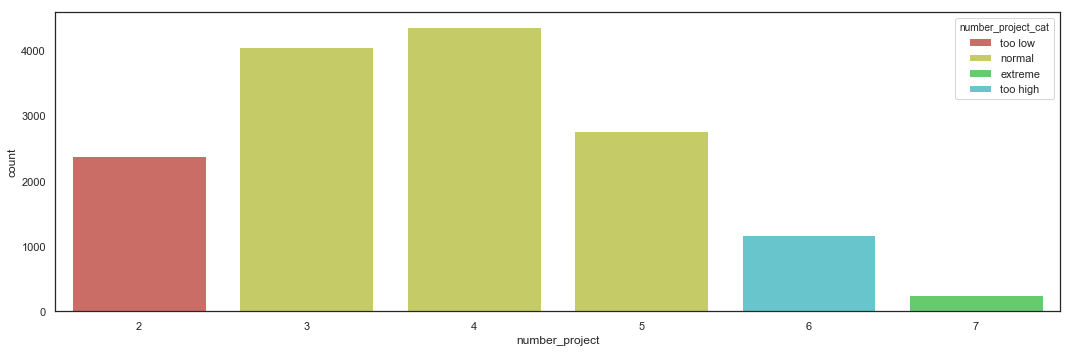
Categorize Number of Projects
Based on the EDA, the Number of Projects can be categorized into 4 categories.
categ = {2:'too low', 3:'normal', 4:'normal', 5:'normal', 6:'too high', 7:'extreme'}
hr_fe['number_project_cat'] = hr_fe.number_project.map(categ)
hr_fe_3['number_project_cat'] = hr_fe_3.number_project.map(categ)
hr_fe_3.number_project_cat.value_counts()
normal      11181
too low      2388
too high     1174
extreme       256
Name: number_project_cat, dtype: int64
plt.figure(figsize=(15,5))
sns.countplot(x=hr_fe_3.number_project,
              hue=hr_fe_3.number_project_cat,
              palette = sns.color_palette("hls", 6),
              dodge = False)
plt.tight_layout()
hr_fe_4 = hr_fe_3.copy()
hr_fe_4 = onehot_encode(hr_fe_4)
hr_fe_4.drop('number_project', inplace=True, axis=1)
X_fe_4, y_fe_4, X_fe_4_train, X_fe_4_test, y_fe_4_train, y_fe_4_test = split_dataset(hr_fe_4, target, split_ratio, seed)
cv_acc(lr, X_fe_4_train, y_fe_4_train, 10, seed)
print()
lr_run(lr, X_fe_4_train, y_fe_4_train, X_fe_4_test, y_fe_4_test)
10-fold cross validation average accuracy: 0.946

Iteration  1 | Accuracy: 0.94
Iteration  2 | Accuracy: 0.94
Iteration  3 | Accuracy: 0.94
Iteration  4 | Accuracy: 0.95
Iteration  5 | Accuracy: 0.96
Iteration  6 | Accuracy: 0.94
Iteration  7 | Accuracy: 0.96
Iteration  8 | Accuracy: 0.96
Iteration  9 | Accuracy: 0.94
Iteration 10 | Accuracy: 0.94

Accuracy on test: 0.950

              precision    recall  f1-score   support

           0       0.96      0.97      0.97      3435
           1       0.90      0.88      0.89      1065

   micro avg       0.95      0.95      0.95      4500
   macro avg       0.93      0.93      0.93      4500
weighted avg       0.95      0.95      0.95      4500

Confusion Matrix:
[[3333  102]
 [ 125  940]]

                                Feature     Coef.
0                            intercept. -2.841608
1                    time_spend_company  0.507726
2                         Work_accident -1.202049
3                 promotion_last_5years -0.838310
4                                salary -0.709500
5                         department_IT -0.031415
6                      department_RandD -0.186888
7                 department_accounting  0.006734
8                         department_hr  0.623972
9                 department_management -0.707609
10                 department_marketing -0.097518
11               department_product_mng -0.202634
12                     department_sales  0.000202
13                   department_support  0.327073
14                 department_technical  0.270137
15  satisfaction_level_bin_(0.00, 0.11]  4.831770
16  satisfaction_level_bin_(0.11, 0.35] -1.270925
17  satisfaction_level_bin_(0.35, 0.46]  2.425227
18  satisfaction_level_bin_(0.46, 0.71] -2.250052
19  satisfaction_level_bin_(0.71, 0.92]  0.187860
20  satisfaction_level_bin_(0.92, 1.00] -3.921827
21     last_evaluation_bin_(0.00, 0.44] -2.975239
22     last_evaluation_bin_(0.44, 0.57]  1.473132
23     last_evaluation_bin_(0.57, 0.76] -0.497719
24     last_evaluation_bin_(0.76, 1.00]  2.001879
25    average_montly_hours_bin_(0, 125] -4.037480
26  average_montly_hours_bin_(125, 131]  0.708746
27  average_montly_hours_bin_(131, 161]  0.080656
28  average_montly_hours_bin_(161, 216] -1.803412
29  average_montly_hours_bin_(216, 274]  0.736018
30  average_montly_hours_bin_(274, 287] -0.077538
31  average_montly_hours_bin_(287, 310]  4.395065
32           number_project_cat_extreme  3.873512
33            number_project_cat_normal -2.153648
34          number_project_cat_too high -1.859092
35           number_project_cat_too low  0.141282
Categorize Time Spent in Company
Based on the EDA, the Time Spent in Company can be categorized into 4 categories, related to the rate of departure.
categ = {2:'low departure', 3:'high departure', 4:'high departure', 5:'very high departure', 6:'high departure', 7:'no departure', 8:'no departure', 10:'no departure'}
hr_fe['time_spend_company_cat'] = hr_fe.time_spend_company.map(categ)
hr_fe_4['time_spend_company_cat'] = hr_fe_4.time_spend_company.map(categ)
hr_fe_4.time_spend_company_cat.value_counts()
high departure         9718
low departure          3244
very high departure    1473
no departure            564
Name: time_spend_company_cat, dtype: int64
plt.figure(figsize=(15,5))
sns.countplot(x=hr_fe_4.time_spend_company,
              hue=hr_fe_4.time_spend_company_cat,
              palette = sns.color_palette("hls", 7),
              dodge = False)
plt.tight_layout()

hr_fe_5 = hr_fe_4.copy()
hr_fe_5 = onehot_encode(hr_fe_5)
hr_fe_5.drop('time_spend_company', inplace=True, axis=1)
X_fe_5, y_fe_5, X_fe_5_train, X_fe_5_test, y_fe_5_train, y_fe_5_test = split_dataset(hr_fe_5, target, split_ratio, seed)
cv_acc(lr, X_fe_5_train, y_fe_5_train, 10, seed)
print()
lr_run(lr, X_fe_5_train, y_fe_5_train, X_fe_5_test, y_fe_5_test)
10-fold cross validation average accuracy: 0.956

Iteration  1 | Accuracy: 0.95
Iteration  2 | Accuracy: 0.94
Iteration  3 | Accuracy: 0.95
Iteration  4 | Accuracy: 0.96
Iteration  5 | Accuracy: 0.96
Iteration  6 | Accuracy: 0.96
Iteration  7 | Accuracy: 0.96
Iteration  8 | Accuracy: 0.96
Iteration  9 | Accuracy: 0.96
Iteration 10 | Accuracy: 0.95

Accuracy on test: 0.956

              precision    recall  f1-score   support

           0       0.96      0.98      0.97      3435
           1       0.93      0.88      0.91      1065

   micro avg       0.96      0.96      0.96      4500
   macro avg       0.95      0.93      0.94      4500
weighted avg       0.96      0.96      0.96      4500

Confusion Matrix:
[[3362   73]
 [ 124  941]]

                                       Feature     Coef.
0                                   intercept. -1.288513
1                                Work_accident -1.210856
2                        promotion_last_5years -0.454837
3                                       salary -0.672500
4                                department_IT -0.235474
5                             department_RandD -0.395298
6                        department_accounting -0.029671
7                                department_hr  0.510471
8                        department_management -0.297698
9                         department_marketing  0.143294
10                      department_product_mng -0.227719
11                            department_sales  0.001829
12                          department_support  0.350340
13                        department_technical  0.179556
14         satisfaction_level_bin_(0.00, 0.11]  5.056556
15         satisfaction_level_bin_(0.11, 0.35] -1.622557
16         satisfaction_level_bin_(0.35, 0.46]  2.196762
17         satisfaction_level_bin_(0.46, 0.71] -1.869052
18         satisfaction_level_bin_(0.71, 0.92]  0.005086
19         satisfaction_level_bin_(0.92, 1.00] -3.767165
20            last_evaluation_bin_(0.00, 0.44] -2.659269
21            last_evaluation_bin_(0.44, 0.57]  1.342359
22            last_evaluation_bin_(0.57, 0.76] -0.295577
23            last_evaluation_bin_(0.76, 1.00]  1.612117
24           average_montly_hours_bin_(0, 125] -4.064773
25         average_montly_hours_bin_(125, 131]  0.755401
26         average_montly_hours_bin_(131, 161]  0.213408
27         average_montly_hours_bin_(161, 216] -1.742236
28         average_montly_hours_bin_(216, 274]  0.596288
29         average_montly_hours_bin_(274, 287]  0.086931
30         average_montly_hours_bin_(287, 310]  4.154612
31                  number_project_cat_extreme  3.500939
32                   number_project_cat_normal -1.998452
33                 number_project_cat_too high -1.610600
34                  number_project_cat_too low  0.107742
35       time_spend_company_cat_high departure  0.357731
36        time_spend_company_cat_low departure -1.265409
37         time_spend_company_cat_no departure -2.014069
38  time_spend_company_cat_very high departure  2.921377
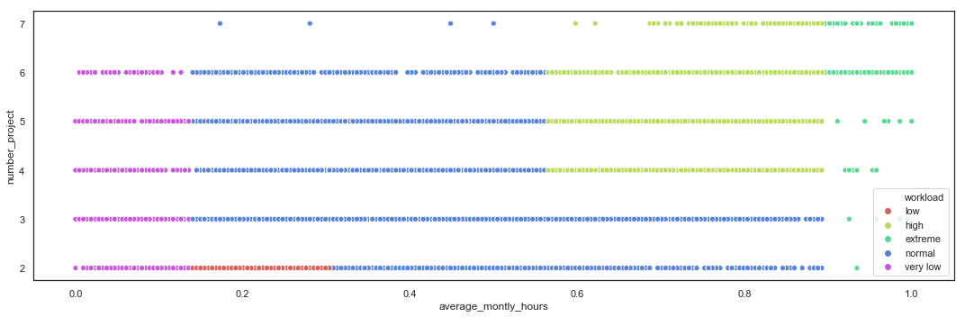
Cluster by Number of Projects and Average Monthly Hours
Based on the EDA, the employees can be clustered by Workload, based on the Number of Projects and Average Monthly Hours, into 5 categories.
def workload_cluster(row):
    if (row['average_montly_hours_bin'] == '(0, 125]'):
        return 'very low'
    if (row['number_project'] <= 2) and (row['average_montly_hours_bin'] in ['(125, 131]','(131, 161]']):
        return 'low'
    if (row['number_project'] >= 4) and (row['average_montly_hours_bin'] in ['(216, 274]','(274, 287]']):
        return 'high'
    if (row['average_montly_hours_bin'] in ['(287, 310]']):
        return 'extreme'
    return 'normal'

hr_fe['workload'] = hr_fe.apply(lambda row: workload_cluster(row), axis=1)
hr_fe.workload.value_counts()
normal      8265
high        4209
low         1709
very low     486
extreme      330
Name: workload, dtype: int64
plt.figure(figsize=(15,5))
sns.scatterplot(x=hr_fe.average_montly_hours,
                y=hr_fe.number_project,
                hue=hr_fe.workload,
                palette = sns.color_palette("hls", 5))
plt.tight_layout()
hr_fe_6 = hr_fe.copy()
hr_fe_6 = onehot_encode(hr_fe_6)
hr_fe_6.drop('satisfaction_level', inplace=True, axis=1)
hr_fe_6.drop('last_evaluation', inplace=True, axis=1)
hr_fe_6.drop('average_montly_hours', inplace=True, axis=1)
hr_fe_6.drop('number_project', inplace=True, axis=1)
hr_fe_6.drop('time_spend_company', inplace=True, axis=1)
X_fe_6, y_fe_6, X_fe_6_train, X_fe_6_test, y_fe_6_train, y_fe_6_test = split_dataset(hr_fe_6, target, split_ratio, seed)
cv_acc(lr, X_fe_6_train, y_fe_6_train, 10, seed)
print()
lr_run(lr, X_fe_6_train, y_fe_6_train, X_fe_6_test, y_fe_6_test)
10-fold cross validation average accuracy: 0.958

Iteration  1 | Accuracy: 0.95
Iteration  2 | Accuracy: 0.94
Iteration  3 | Accuracy: 0.95
Iteration  4 | Accuracy: 0.96
Iteration  5 | Accuracy: 0.97
Iteration  6 | Accuracy: 0.96
Iteration  7 | Accuracy: 0.96
Iteration  8 | Accuracy: 0.97
Iteration  9 | Accuracy: 0.96
Iteration 10 | Accuracy: 0.95

Accuracy on test: 0.959

              precision    recall  f1-score   support

           0       0.96      0.98      0.97      3435
           1       0.94      0.88      0.91      1065

   micro avg       0.96      0.96      0.96      4500
   macro avg       0.95      0.93      0.94      4500
weighted avg       0.96      0.96      0.96      4500

Confusion Matrix:
[[3377   58]
 [ 125  940]]

                                       Feature     Coef.
0                                   intercept. -0.766901
1                                Work_accident -1.173201
2                        promotion_last_5years -0.439302
3                                       salary -0.662271
4                                department_IT -0.297131
5                             department_RandD -0.447797
6                        department_accounting  0.000741
7                                department_hr  0.458777
8                        department_management -0.164455
9                         department_marketing  0.048457
10                      department_product_mng -0.187570
11                            department_sales  0.034650
12                          department_support  0.347782
13                        department_technical  0.205697
14                            workload_extreme  2.350234
15                               workload_high  0.104323
16                                workload_low  1.471144
17                             workload_normal -1.650481
18                           workload_very low -2.276069
19       time_spend_company_cat_high departure  0.289188
20        time_spend_company_cat_low departure -1.110152
21         time_spend_company_cat_no departure -1.839473
22  time_spend_company_cat_very high departure  2.659588
23           average_montly_hours_bin_(0, 125] -2.276069
24         average_montly_hours_bin_(125, 131]  0.579145
25         average_montly_hours_bin_(131, 161]  0.135179
26         average_montly_hours_bin_(161, 216] -0.624238
27         average_montly_hours_bin_(216, 274] -0.014268
28         average_montly_hours_bin_(274, 287] -0.150833
29         average_montly_hours_bin_(287, 310]  2.350234
30            last_evaluation_bin_(0.00, 0.44] -2.541263
31            last_evaluation_bin_(0.44, 0.57]  1.163123
32            last_evaluation_bin_(0.57, 0.76] -0.196012
33            last_evaluation_bin_(0.76, 1.00]  1.573302
34                  number_project_cat_extreme  3.487829
35                   number_project_cat_normal -1.632124
36                 number_project_cat_too high -1.306443
37                  number_project_cat_too low -0.550112
38         satisfaction_level_bin_(0.00, 0.11]  4.765909
39         satisfaction_level_bin_(0.11, 0.35] -1.400822
40         satisfaction_level_bin_(0.35, 0.46]  1.637670
41         satisfaction_level_bin_(0.46, 0.71] -1.633800
42         satisfaction_level_bin_(0.71, 0.92]  0.169115
43         satisfaction_level_bin_(0.92, 1.00] -3.538921
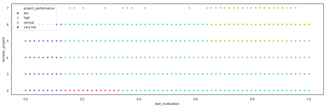
Cluster by Number of Projects and Last Evaluation
Based on the EDA, the employees can be clustered by Project Performance, based on the Number of Projects and Last Evaluation, into 4 categories.
def project_performance_cluster(row):
    if (row['last_evaluation_bin'] == '(0.00, 0.44]'):
        return 'very low'
    if (row['number_project'] <= 2) and (row['last_evaluation_bin'] in ['(0.44, 0.57]']):
        return 'low'
    if (row['number_project'] >= 4) and (row['last_evaluation_bin'] in ['(0.76, 1.00]']):
        return 'high'
    return 'normal'

hr_fe['project_performance'] = hr_fe.apply(lambda row: project_performance_cluster(row), axis=1)
hr_fe.project_performance.value_counts()
normal      8245
high        4589
low         1720
very low     445
Name: project_performance, dtype: int64
plt.figure(figsize=(15,5))
sns.scatterplot(x=hr_fe.last_evaluation,
                y=hr_fe.number_project,
                hue=hr_fe.project_performance,
                palette = sns.color_palette("hls", 4))
plt.tight_layout()
hr_fe_7 = hr_fe.copy()
hr_fe_7 = onehot_encode(hr_fe_7)
hr_fe_7.drop('satisfaction_level', inplace=True, axis=1)
hr_fe_7.drop('last_evaluation', inplace=True, axis=1)
hr_fe_7.drop('average_montly_hours', inplace=True, axis=1)
hr_fe_7.drop('number_project', inplace=True, axis=1)
hr_fe_7.drop('time_spend_company', inplace=True, axis=1)
X_fe_7, y_fe_7, X_fe_7_train, X_fe_7_test, y_fe_7_train, y_fe_7_test = split_dataset(hr_fe_7, target, split_ratio, seed)
cv_acc(lr, X_fe_7_train, y_fe_7_train, 10, seed)
print()
lr_run(lr, X_fe_7_train, y_fe_7_train, X_fe_7_test, y_fe_7_test)
10-fold cross validation average accuracy: 0.960

Iteration  1 | Accuracy: 0.96
Iteration  2 | Accuracy: 0.95
Iteration  3 | Accuracy: 0.96
Iteration  4 | Accuracy: 0.96
Iteration  5 | Accuracy: 0.97
Iteration  6 | Accuracy: 0.96
Iteration  7 | Accuracy: 0.96
Iteration  8 | Accuracy: 0.96
Iteration  9 | Accuracy: 0.96
Iteration 10 | Accuracy: 0.95

Accuracy on test: 0.958

              precision    recall  f1-score   support

           0       0.96      0.98      0.97      3435
           1       0.93      0.88      0.91      1065

   micro avg       0.96      0.96      0.96      4500
   macro avg       0.95      0.93      0.94      4500
weighted avg       0.96      0.96      0.96      4500

Confusion Matrix:
[[3368   67]
 [ 123  942]]

                                       Feature     Coef.
0                                   intercept. -0.304227
1                                Work_accident -1.223252
2                        promotion_last_5years -0.510657
3                                       salary -0.639244
4                                department_IT -0.308566
5                             department_RandD -0.427170
6                        department_accounting -0.113093
7                                department_hr  0.396920
8                        department_management -0.146822
9                         department_marketing  0.112515
10                      department_product_mng -0.140261
11                            department_sales  0.023193
12                          department_support  0.369251
13                        department_technical  0.234417
14                            workload_extreme  2.405614
15                               workload_high -0.219293
16                                workload_low  1.266443
17                             workload_normal -1.301441
18                           workload_very low -2.150941
19       time_spend_company_cat_high departure  0.299676
20        time_spend_company_cat_low departure -1.065227
21         time_spend_company_cat_no departure -1.923445
22  time_spend_company_cat_very high departure  2.689379
23           average_montly_hours_bin_(0, 125] -2.150941
24         average_montly_hours_bin_(125, 131]  0.310555
25         average_montly_hours_bin_(131, 161] -0.065836
26         average_montly_hours_bin_(161, 216] -0.782745
27         average_montly_hours_bin_(216, 274]  0.117264
28         average_montly_hours_bin_(274, 287]  0.166471
29         average_montly_hours_bin_(287, 310]  2.405614
30            last_evaluation_bin_(0.00, 0.44] -1.472612
31            last_evaluation_bin_(0.44, 0.57]  0.498097
32            last_evaluation_bin_(0.57, 0.76]  0.165295
33            last_evaluation_bin_(0.76, 1.00]  0.809603
34                    project_performance_high  0.246351
35                     project_performance_low  2.100090
36                  project_performance_normal -0.873446
37                project_performance_very low -1.472612
38                  number_project_cat_extreme  3.644086
39                   number_project_cat_normal -1.391861
40                 number_project_cat_too high -1.002857
41                  number_project_cat_too low -1.248984
42         satisfaction_level_bin_(0.00, 0.11]  4.679780
43         satisfaction_level_bin_(0.11, 0.35] -1.331063
44         satisfaction_level_bin_(0.35, 0.46]  1.205874
45         satisfaction_level_bin_(0.46, 0.71] -1.514709
46         satisfaction_level_bin_(0.71, 0.92]  0.241973
47         satisfaction_level_bin_(0.92, 1.00] -3.281472
Cluster by Last Evaluation and Average Monthly Hours
Based on the EDA, the employees can be clustered by Efficiency, based on the Last Evaluation and the Average Monthly Hours, into 4 categories.
def efficiency_cluster(row):
    if (row['last_evaluation_bin'] == '(0.00, 0.44]'):
        return 'very low'
    if (row['average_montly_hours_bin'] in ['(0, 125]']):
        return 'very low'
    if (row['last_evaluation_bin'] in ['(0.44, 0.57]']) and (row['average_montly_hours_bin'] in ['(125, 131]', '(131, 161]']):
        return 'low'
    if (row['last_evaluation_bin'] in ['(0.76, 1.00]']) and (row['average_montly_hours_bin'] in ['(216, 274]', '(274, 287]','(287, 310]']):
        return 'high'
    return 'normal'

hr_fe['efficiency'] = hr_fe.apply(lambda row: efficiency_cluster(row), axis=1)
hr_fe.efficiency.value_counts()
normal      8436
high        3719
low         1994
very low     850
Name: efficiency, dtype: int64
plt.figure(figsize=(15,5))
sns.scatterplot(x=hr_fe.average_montly_hours,
                y=hr_fe.last_evaluation,
                hue=hr_fe.efficiency,
                palette = sns.color_palette("hls", 4))
plt.tight_layout()

hr_fe_8 = hr_fe.copy()
hr_fe_8 = onehot_encode(hr_fe_8)
hr_fe_8.drop('satisfaction_level', inplace=True, axis=1)
hr_fe_8.drop('last_evaluation', inplace=True, axis=1)
hr_fe_8.drop('average_montly_hours', inplace=True, axis=1)
hr_fe_8.drop('number_project', inplace=True, axis=1)
hr_fe_8.drop('time_spend_company', inplace=True, axis=1)
X_fe_8, y_fe_8, X_fe_8_train, X_fe_8_test, y_fe_8_train, y_fe_8_test = split_dataset(hr_fe_8, target, split_ratio, seed)
cv_acc(lr, X_fe_8_train, y_fe_8_train, 10, seed)
print()
lr_run(lr, X_fe_8_train, y_fe_8_train, X_fe_8_test, y_fe_8_test)
10-fold cross validation average accuracy: 0.960

Iteration  1 | Accuracy: 0.96
Iteration  2 | Accuracy: 0.95
Iteration  3 | Accuracy: 0.96
Iteration  4 | Accuracy: 0.96
Iteration  5 | Accuracy: 0.97
Iteration  6 | Accuracy: 0.96
Iteration  7 | Accuracy: 0.96
Iteration  8 | Accuracy: 0.96
Iteration  9 | Accuracy: 0.96
Iteration 10 | Accuracy: 0.95

Accuracy on test: 0.960

              precision    recall  f1-score   support

           0       0.96      0.98      0.97      3435
           1       0.94      0.88      0.91      1065

   micro avg       0.96      0.96      0.96      4500
   macro avg       0.95      0.93      0.94      4500
weighted avg       0.96      0.96      0.96      4500

Confusion Matrix:
[[3377   58]
 [ 124  941]]

                                       Feature     Coef.
0                                   intercept.  0.110311
1                                Work_accident -1.234954
2                        promotion_last_5years -0.581323
3                                       salary -0.653274
4                                department_IT -0.319980
5                             department_RandD -0.444509
6                        department_accounting -0.118532
7                                department_hr  0.420489
8                        department_management -0.156571
9                         department_marketing  0.097993
10                      department_product_mng -0.141090
11                            department_sales  0.034649
12                          department_support  0.373496
13                        department_technical  0.253988
14                            workload_extreme  2.378101
15                               workload_high -0.310825
16                                workload_low  0.498770
17                             workload_normal -1.224138
18                           workload_very low -1.341976
19       time_spend_company_cat_high departure  0.291586
20        time_spend_company_cat_low departure -1.079268
21         time_spend_company_cat_no departure -1.877955
22  time_spend_company_cat_very high departure  2.665570
23           average_montly_hours_bin_(0, 125] -1.341976
24         average_montly_hours_bin_(125, 131]  0.122886
25         average_montly_hours_bin_(131, 161] -0.304675
26         average_montly_hours_bin_(161, 216] -0.571684
27         average_montly_hours_bin_(216, 274] -0.235870
28         average_montly_hours_bin_(274, 287] -0.046850
29         average_montly_hours_bin_(287, 310]  2.378101
30            last_evaluation_bin_(0.00, 0.44] -0.789941
31            last_evaluation_bin_(0.44, 0.57]  0.075586
32            last_evaluation_bin_(0.57, 0.76]  0.324766
33            last_evaluation_bin_(0.76, 1.00]  0.389521
34                    project_performance_high  0.179345
35                     project_performance_low  1.434834
36                  project_performance_normal -0.824305
37                project_performance_very low -0.789941
38                  number_project_cat_extreme  3.511605
39                   number_project_cat_normal -1.541114
40                 number_project_cat_too high -1.025555
41                  number_project_cat_too low -0.945003
42         satisfaction_level_bin_(0.00, 0.11]  4.547035
43         satisfaction_level_bin_(0.11, 0.35] -1.297088
44         satisfaction_level_bin_(0.35, 0.46]  1.129828
45         satisfaction_level_bin_(0.46, 0.71] -1.465960
46         satisfaction_level_bin_(0.71, 0.92]  0.271559
47         satisfaction_level_bin_(0.92, 1.00] -3.185440
48                             efficiency_high  0.730403
49                              efficiency_low  1.642109
50                           efficiency_normal -0.284602
51                         efficiency_very low -2.087977
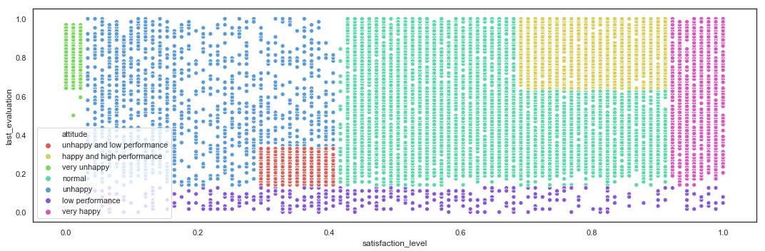
Cluster by Last Evaluation and Satisfaction Level
Based on the EDA, the employees can be clustered by Attitude, based on the Last Evaluation and the Satisfaction Level, into 7 categories.
def attitude_cluster(row):
    if (row['last_evaluation_bin'] == '(0.00, 0.44]'):
        return 'low performance'
    if (row['satisfaction_level_bin'] in ['(0.92, 1.00]']):
        return 'very happy'
    if (row['last_evaluation_bin'] in ['(0.76, 1.00]']) and (row['satisfaction_level_bin'] in ['(0.71, 0.92]']):
        return 'happy and high performance'
    if (row['last_evaluation_bin'] in ['(0.44, 0.57]']) and (row['satisfaction_level_bin'] in ['(0.35, 0.46]']):
        return 'unhappy and low performance'
    if (row['satisfaction_level_bin'] in ['(0.00, 0.11]']):
        return 'very unhappy'
    if (row['satisfaction_level_bin'] in ['(0.11, 0.35]','(0.35, 0.46]']):
        return 'unhappy'
    return 'normal'

hr_fe['attitude'] = hr_fe.apply(lambda row: attitude_cluster(row), axis=1)
hr_fe.attitude.value_counts()
normal                         6668
happy and high performance     2553
unhappy and low performance    1635
unhappy                        1474
very happy                     1336
very unhappy                    888
low performance                 445
Name: attitude, dtype: int64
plt.figure(figsize=(15,5))
sns.scatterplot(x=hr_fe.satisfaction_level,
                y=hr_fe.last_evaluation,
                hue=hr_fe.attitude,
                palette = sns.color_palette("hls", 7))
plt.tight_layout()
hr_fe_9 = hr_fe.copy()
hr_fe_9 = onehot_encode(hr_fe_9)
hr_fe_9.drop('satisfaction_level', inplace=True, axis=1)
hr_fe_9.drop('last_evaluation', inplace=True, axis=1)
hr_fe_9.drop('average_montly_hours', inplace=True, axis=1)
hr_fe_9.drop('number_project', inplace=True, axis=1)
hr_fe_9.drop('time_spend_company', inplace=True, axis=1)
X_fe_9, y_fe_9, X_fe_9_train, X_fe_9_test, y_fe_9_train, y_fe_9_test = split_dataset(hr_fe_9, target, split_ratio, seed)
cv_acc(lr, X_fe_9_train, y_fe_9_train, 10, seed)
print()
lr_run(lr, X_fe_9_train, y_fe_9_train, X_fe_9_test, y_fe_9_test)
10-fold cross validation average accuracy: 0.964

Iteration  1 | Accuracy: 0.96
Iteration  2 | Accuracy: 0.95
Iteration  3 | Accuracy: 0.96
Iteration  4 | Accuracy: 0.97
Iteration  5 | Accuracy: 0.97
Iteration  6 | Accuracy: 0.97
Iteration  7 | Accuracy: 0.97
Iteration  8 | Accuracy: 0.96
Iteration  9 | Accuracy: 0.96
Iteration 10 | Accuracy: 0.96

Accuracy on test: 0.964

              precision    recall  f1-score   support

           0       0.97      0.98      0.98      3435
           1       0.94      0.90      0.92      1065

   micro avg       0.96      0.96      0.96      4500
   macro avg       0.96      0.94      0.95      4500
weighted avg       0.96      0.96      0.96      4500

Confusion Matrix:
[[3379   56]
 [ 108  957]]

                                       Feature     Coef.
0                                   intercept.  0.155602
1                                Work_accident -1.143174
2                        promotion_last_5years -0.597843
3                                       salary -0.652169
4                                department_IT -0.355823
5                             department_RandD -0.441450
6                        department_accounting -0.095917
7                                department_hr  0.447624
8                        department_management -0.163427
9                         department_marketing  0.093569
10                      department_product_mng -0.171977
11                            department_sales  0.034884
12                          department_support  0.366134
13                        department_technical  0.288470
14                            workload_extreme  2.282292
15                               workload_high -0.227062
16                                workload_low  0.383963
17                             workload_normal -1.056297
18                           workload_very low -1.380807
19       time_spend_company_cat_high departure  0.258945
20        time_spend_company_cat_low departure -1.051914
21         time_spend_company_cat_no departure -1.793281
22  time_spend_company_cat_very high departure  2.588338
23           average_montly_hours_bin_(0, 125] -1.380807
24         average_montly_hours_bin_(125, 131]  0.087262
25         average_montly_hours_bin_(131, 161] -0.283742
26         average_montly_hours_bin_(161, 216] -0.697097
27         average_montly_hours_bin_(216, 274] -0.167288
28         average_montly_hours_bin_(274, 287]  0.161469
29         average_montly_hours_bin_(287, 310]  2.282292
30            last_evaluation_bin_(0.00, 0.44] -0.693405
31            last_evaluation_bin_(0.44, 0.57]  0.121621
32            last_evaluation_bin_(0.57, 0.76]  0.748939
33            last_evaluation_bin_(0.76, 1.00] -0.175065
34         attitude_happy and high performance  0.807235
35                    attitude_low performance -0.693405
36                             attitude_normal -1.154903
37                            attitude_unhappy -1.048762
38        attitude_unhappy and low performance  1.378160
39                         attitude_very happy -1.938233
40                       attitude_very unhappy  2.651998
41                    project_performance_high  0.419734
42                     project_performance_low  0.855019
43                  project_performance_normal -0.579259
44                project_performance_very low -0.693405
45                  number_project_cat_extreme  3.202322
46                   number_project_cat_normal -1.490338
47                 number_project_cat_too high -0.978540
48                  number_project_cat_too low -0.731354
49         satisfaction_level_bin_(0.00, 0.11]  2.651998
50         satisfaction_level_bin_(0.11, 0.35] -0.522950
51         satisfaction_level_bin_(0.35, 0.46]  0.552467
52         satisfaction_level_bin_(0.46, 0.71] -0.530850
53         satisfaction_level_bin_(0.71, 0.92] -0.200445
54         satisfaction_level_bin_(0.92, 1.00] -1.948131
55                             efficiency_high  0.631356
56                              efficiency_low  1.559049
57                           efficiency_normal -0.140877
58                         efficiency_very low -2.047439
Removing Unbinned Variables and Encoding New Features
The variables which have been binned are removed from the dataset, and new features are one hot encoded.
hr_fe_encoded = onehot_encode(hr_fe)
hr_fe_encoded.drop('satisfaction_level', inplace=True, axis=1)
hr_fe_encoded.drop('last_evaluation', inplace=True, axis=1)
hr_fe_encoded.drop('average_montly_hours', inplace=True, axis=1)
hr_fe_encoded.drop('number_project', inplace=True, axis=1)
hr_fe_encoded.drop('time_spend_company', inplace=True, axis=1)
df_desc(hr_fe_encoded)
| dtype | NAs | Numerical | Boolean | Categorical | |
|---|---|---|---|---|---|
| Work_accident | int64 | 0 | False | True | False |
| left | int64 | 0 | False | True | False |
| promotion_last_5years | int64 | 0 | False | True | False |
| salary | int64 | 0 | True | False | False |
| department_IT | uint8 | 0 | False | True | False |
| department_RandD | uint8 | 0 | False | True | False |
| department_accounting | uint8 | 0 | False | True | False |
| department_hr | uint8 | 0 | False | True | False |
| department_management | uint8 | 0 | False | True | False |
| department_marketing | uint8 | 0 | False | True | False |
| department_product_mng | uint8 | 0 | False | True | False |
| department_sales | uint8 | 0 | False | True | False |
| department_support | uint8 | 0 | False | True | False |
| department_technical | uint8 | 0 | False | True | False |
| workload_extreme | uint8 | 0 | False | True | False |
| workload_high | uint8 | 0 | False | True | False |
| workload_low | uint8 | 0 | False | True | False |
| workload_normal | uint8 | 0 | False | True | False |
| workload_very low | uint8 | 0 | False | True | False |
| time_spend_company_cat_high departure | uint8 | 0 | False | True | False |
| time_spend_company_cat_low departure | uint8 | 0 | False | True | False |
| time_spend_company_cat_no departure | uint8 | 0 | False | True | False |
| time_spend_company_cat_very high departure | uint8 | 0 | False | True | False |
| average_montly_hours_bin_(0, 125] | uint8 | 0 | False | True | False |
| average_montly_hours_bin_(125, 131] | uint8 | 0 | False | True | False |
| average_montly_hours_bin_(131, 161] | uint8 | 0 | False | True | False |
| average_montly_hours_bin_(161, 216] | uint8 | 0 | False | True | False |
| average_montly_hours_bin_(216, 274] | uint8 | 0 | False | True | False |
| average_montly_hours_bin_(274, 287] | uint8 | 0 | False | True | False |
| average_montly_hours_bin_(287, 310] | uint8 | 0 | False | True | False |
| last_evaluation_bin_(0.00, 0.44] | uint8 | 0 | False | True | False |
| last_evaluation_bin_(0.44, 0.57] | uint8 | 0 | False | True | False |
| last_evaluation_bin_(0.57, 0.76] | uint8 | 0 | False | True | False |
| last_evaluation_bin_(0.76, 1.00] | uint8 | 0 | False | True | False |
| attitude_happy and high performance | uint8 | 0 | False | True | False |
| attitude_low performance | uint8 | 0 | False | True | False |
| attitude_normal | uint8 | 0 | False | True | False |
| attitude_unhappy | uint8 | 0 | False | True | False |
| attitude_unhappy and low performance | uint8 | 0 | False | True | False |
| attitude_very happy | uint8 | 0 | False | True | False |
| attitude_very unhappy | uint8 | 0 | False | True | False |
| project_performance_high | uint8 | 0 | False | True | False |
| project_performance_low | uint8 | 0 | False | True | False |
| project_performance_normal | uint8 | 0 | False | True | False |
| project_performance_very low | uint8 | 0 | False | True | False |
| number_project_cat_extreme | uint8 | 0 | False | True | False |
| number_project_cat_normal | uint8 | 0 | False | True | False |
| number_project_cat_too high | uint8 | 0 | False | True | False |
| number_project_cat_too low | uint8 | 0 | False | True | False |
| satisfaction_level_bin_(0.00, 0.11] | uint8 | 0 | False | True | False |
| satisfaction_level_bin_(0.11, 0.35] | uint8 | 0 | False | True | False |
| satisfaction_level_bin_(0.35, 0.46] | uint8 | 0 | False | True | False |
| satisfaction_level_bin_(0.46, 0.71] | uint8 | 0 | False | True | False |
| satisfaction_level_bin_(0.71, 0.92] | uint8 | 0 | False | True | False |
| satisfaction_level_bin_(0.92, 1.00] | uint8 | 0 | False | True | False |
| efficiency_high | uint8 | 0 | False | True | False |
| efficiency_low | uint8 | 0 | False | True | False |
| efficiency_normal | uint8 | 0 | False | True | False |
| efficiency_very low | uint8 | 0 | False | True | False |
Features Selection
The dataset resulting from the Feature Engineering phase contains 58 features, with a model reaching the accuracy of 0.964. The Feature Selection phase aims to reduce the number of variables used by the model.
X_fe_encoded, y_fe_encoded, X_fe_encoded_train, X_fe_encoded_test, y_fe_encoded_train, y_fe_encoded_test = split_dataset(hr_fe_encoded, target, split_ratio, seed)
cv_acc(lr, X_fe_encoded_train, y_fe_encoded_train, 10, seed)
print()
lr_run(lr, X_fe_encoded_train, y_fe_encoded_train, X_fe_encoded_test, y_fe_encoded_test)
10-fold cross validation average accuracy: 0.964

Iteration  1 | Accuracy: 0.96
Iteration  2 | Accuracy: 0.95
Iteration  3 | Accuracy: 0.96
Iteration  4 | Accuracy: 0.97
Iteration  5 | Accuracy: 0.97
Iteration  6 | Accuracy: 0.97
Iteration  7 | Accuracy: 0.97
Iteration  8 | Accuracy: 0.96
Iteration  9 | Accuracy: 0.96
Iteration 10 | Accuracy: 0.96

Accuracy on test: 0.964

              precision    recall  f1-score   support

           0       0.97      0.98      0.98      3435
           1       0.94      0.90      0.92      1065

   micro avg       0.96      0.96      0.96      4500
   macro avg       0.96      0.94      0.95      4500
weighted avg       0.96      0.96      0.96      4500

Confusion Matrix:
[[3379   56]
 [ 108  957]]

                                       Feature     Coef.
0                                   intercept.  0.155602
1                                Work_accident -1.143174
2                        promotion_last_5years -0.597843
3                                       salary -0.652169
4                                department_IT -0.355823
5                             department_RandD -0.441450
6                        department_accounting -0.095917
7                                department_hr  0.447624
8                        department_management -0.163427
9                         department_marketing  0.093569
10                      department_product_mng -0.171977
11                            department_sales  0.034884
12                          department_support  0.366134
13                        department_technical  0.288470
14                            workload_extreme  2.282292
15                               workload_high -0.227062
16                                workload_low  0.383963
17                             workload_normal -1.056297
18                           workload_very low -1.380807
19       time_spend_company_cat_high departure  0.258945
20        time_spend_company_cat_low departure -1.051914
21         time_spend_company_cat_no departure -1.793281
22  time_spend_company_cat_very high departure  2.588338
23           average_montly_hours_bin_(0, 125] -1.380807
24         average_montly_hours_bin_(125, 131]  0.087262
25         average_montly_hours_bin_(131, 161] -0.283742
26         average_montly_hours_bin_(161, 216] -0.697097
27         average_montly_hours_bin_(216, 274] -0.167288
28         average_montly_hours_bin_(274, 287]  0.161469
29         average_montly_hours_bin_(287, 310]  2.282292
30            last_evaluation_bin_(0.00, 0.44] -0.693405
31            last_evaluation_bin_(0.44, 0.57]  0.121621
32            last_evaluation_bin_(0.57, 0.76]  0.748939
33            last_evaluation_bin_(0.76, 1.00] -0.175065
34         attitude_happy and high performance  0.807235
35                    attitude_low performance -0.693405
36                             attitude_normal -1.154903
37                            attitude_unhappy -1.048762
38        attitude_unhappy and low performance  1.378160
39                         attitude_very happy -1.938233
40                       attitude_very unhappy  2.651998
41                    project_performance_high  0.419734
42                     project_performance_low  0.855019
43                  project_performance_normal -0.579259
44                project_performance_very low -0.693405
45                  number_project_cat_extreme  3.202322
46                   number_project_cat_normal -1.490338
47                 number_project_cat_too high -0.978540
48                  number_project_cat_too low -0.731354
49         satisfaction_level_bin_(0.00, 0.11]  2.651998
50         satisfaction_level_bin_(0.11, 0.35] -0.522950
51         satisfaction_level_bin_(0.35, 0.46]  0.552467
52         satisfaction_level_bin_(0.46, 0.71] -0.530850
53         satisfaction_level_bin_(0.71, 0.92] -0.200445
54         satisfaction_level_bin_(0.92, 1.00] -1.948131
55                             efficiency_high  0.631356
56                              efficiency_low  1.559049
57                           efficiency_normal -0.140877
58                         efficiency_very low -2.047439
plot_roc(lr, X_fe_encoded_test, y_fe_encoded_test)

The Recursive Feature Elimination (RFE) method is used to select the most relevant features for the model.
accuracies = pd.DataFrame(columns=['features','accuracy', 'cols'])
print('Iterations:')

for i in range(1, len(X_fe_encoded.columns)+1):
    logreg = LogisticRegression(solver='lbfgs', max_iter=250)
    rfe = RFE(logreg, i)
    rfe = rfe.fit(X_fe_encoded, y_fe_encoded.values.ravel())

    cols_rfe = list(X_fe_encoded.loc[:, rfe.support_])
    X_rfe_sel = X_fe_encoded_train[cols_rfe]
    X_rfe_test_sel = X_fe_encoded_test[cols_rfe]

    result = logreg.fit(X_rfe_sel, y_fe_encoded_train.values.ravel())
    acc_test = logreg.score(X_rfe_test_sel, y_fe_encoded_test)

    accuracies.loc[i] = [i, acc_test, cols_rfe]
    print(i, end='   ')
Iterations:
1   2   3   4   5   6   7   8   9   10   11   12   13   14   15   16   17   18   19   20   21   22   23   24   25   26   27   28   29   30   31   32   33   34   35   36   37   38   39   40   41   42   43   44   45   46   47   48   49   50   51   52   53   54   55   56   57   58
# Line Plot
plt.figure(figsize=(15,5))
sns.lineplot(x = accuracies['features'],
             y = accuracies['accuracy'],
             color = 'steelblue')#.axes.set_xlim(min(hr.last_evaluation),max(hr.last_evaluation))
plt.tight_layout()
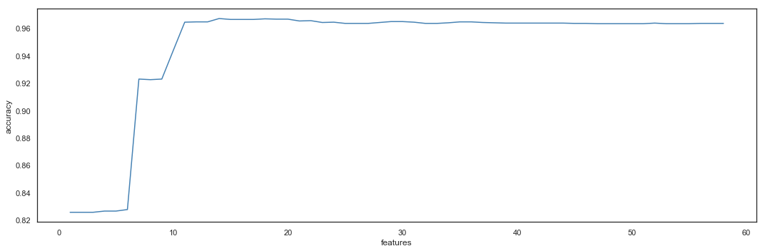
accuracies.nlargest(10, 'accuracy')
| features | accuracy | cols | |
|---|---|---|---|
| 14 | 14 | 0.967111 | [workload_extreme, workload_normal, time_spend... |
| 18 | 18 | 0.966889 | [workload_extreme, workload_normal, time_spend... |
| 19 | 19 | 0.966667 | [workload_extreme, workload_normal, workload_v... |
| 20 | 20 | 0.966667 | [Work_accident, workload_extreme, workload_nor... |
| 15 | 15 | 0.966444 | [workload_extreme, workload_normal, time_spend... |
| 16 | 16 | 0.966444 | [workload_extreme, workload_normal, time_spend... |
| 17 | 17 | 0.966444 | [workload_extreme, workload_normal, time_spend... |
| 22 | 22 | 0.965556 | [Work_accident, workload_extreme, workload_nor... |
| 21 | 21 | 0.965333 | [Work_accident, workload_extreme, workload_nor... |
| 29 | 29 | 0.964889 | [Work_accident, promotion_last_5years, workloa... |
The best model is found with 14 features, for an accuracy of 0.967.
from sklearn.exceptions import ConvergenceWarning
import warnings
warnings.filterwarnings(action='ignore', category=ConvergenceWarning)

features_rfe = list(hr_fe_encoded)
features_rfe.remove(target)

X_rfe = hr_fe_encoded.loc[:, features_rfe]
y_rfe = hr_fe_encoded.loc[:, target]

logreg = LogisticRegression(solver='lbfgs', max_iter=250)
rfe = RFE(logreg, accuracies.nlargest(1,'accuracy').features.values.ravel()[0])
rfe = rfe.fit(X_rfe, y_rfe)

print(sum(rfe.support_),'selected features:')
for i in list(X_rfe.loc[:, rfe.support_]):
    print(i)
14 selected features:
workload_extreme
workload_normal
time_spend_company_cat_no departure
time_spend_company_cat_very high departure
average_montly_hours_bin_(287, 310]
attitude_normal
attitude_unhappy
attitude_very happy
attitude_very unhappy
number_project_cat_extreme
satisfaction_level_bin_(0.00, 0.11]
satisfaction_level_bin_(0.92, 1.00]
efficiency_low
efficiency_very low
Final Metric
Initial Dataset
A final model is tested with the 14 selected features.
cols = list(X_rfe.loc[:, rfe.support_]) + [target]
hr_sel = hr_fe_encoded[cols]
X_sel, y_sel, X_sel_train, X_sel_test, y_sel_train, y_sel_test = split_dataset(hr_sel, target, split_ratio, seed)
cv_acc(lr, X_sel_train, y_sel_train, 10, seed)
print()
lr_run(lr, X_sel_train, y_sel_train, X_sel_test, y_sel_test)
10-fold cross validation average accuracy: 0.964

Iteration  1 | Accuracy: 0.96
Iteration  2 | Accuracy: 0.95
Iteration  3 | Accuracy: 0.96
Iteration  4 | Accuracy: 0.97
Iteration  5 | Accuracy: 0.97
Iteration  6 | Accuracy: 0.96
Iteration  7 | Accuracy: 0.98
Iteration  8 | Accuracy: 0.97
Iteration  9 | Accuracy: 0.96
Iteration 10 | Accuracy: 0.95

Accuracy on test: 0.967

              precision    recall  f1-score   support

           0       0.96      1.00      0.98      3435
           1       0.98      0.88      0.93      1065

   micro avg       0.97      0.97      0.97      4500
   macro avg       0.97      0.94      0.95      4500
weighted avg       0.97      0.97      0.97      4500

Confusion Matrix:
[[3419   16]
 [ 132  933]]

                                       Feature     Coef.
0                                   intercept. -0.375952
1                             workload_extreme  2.245120
2                              workload_normal -2.183617
3          time_spend_company_cat_no departure -2.016273
4   time_spend_company_cat_very high departure  2.403233
5          average_montly_hours_bin_(287, 310]  2.245120
6                              attitude_normal -2.936478
7                             attitude_unhappy -2.295986
8                          attitude_very happy -2.423485
9                        attitude_very unhappy  2.582233
10                  number_project_cat_extreme  3.987229
11         satisfaction_level_bin_(0.00, 0.11]  2.582233
12         satisfaction_level_bin_(0.92, 1.00] -2.448987
13                              efficiency_low  3.295257
14                         efficiency_very low -4.182167
plot_roc(lr, X_sel_test, y_sel_test)

The model returns the accuracy of 0.967. The recall for employees who left the company now reaches 88%, which will allow the management to better predict which employees have a high probability to leave.
Over Sampling with SMOTE
To ensure the model is not biased by the imbalanced proportions of the variable left, the dataset is enriched by synthetic samples using the Synthetic Minority Oversampling Technique (SMOTE). Only the train set is over-sampled, to ensure it doesn’t get polluted by the test set.
# Install the imbalanced-learn package with this command:
# conda install -c conda-forge imbalanced-learn
from imblearn.over_sampling import SMOTE

os = SMOTE(random_state=0)
X_smote, y_smote, X_smote_train, X_smote_test, y_smote_train, y_smote_test = split_dataset(hr_fe_encoded, target, split_ratio, seed)
columns = X_smote_train.columns

os_data_X,os_data_y = os.fit_sample(X_smote_train, y_smote_train.values.ravel())
os_data_X = pd.DataFrame(data=os_data_X, columns=columns)
os_data_y= pd.DataFrame(data=os_data_y,columns=['left'])
# we can Check the numbers of our data
print("Length of oversampled data is ",len(os_data_X))
print("Number of 'stayed' in oversampled data",len(os_data_y[os_data_y['left']==0]))
print("Number of 'left'",len(os_data_y[os_data_y['left']==1]))
print("Proportion of 'stayed' data in oversampled data is ",len(os_data_y[os_data_y['left']==0])/len(os_data_X))
print("Proportion of 'left' data in oversampled data is ",len(os_data_y[os_data_y['left']==1])/len(os_data_X))
Length of oversampled data is  15986
Number of 'stayed' in oversampled data 7993
Number of 'left' 7993
Proportion of 'stayed' data in oversampled data is  0.5
Proportion of 'left' data in oversampled data is  0.5
cv_acc(lr, os_data_X, os_data_y, 10, seed)
print()
lr_run(lr, os_data_X, os_data_y, X_smote_test, y_smote_test)
10-fold cross validation average accuracy: 0.963

Iteration  1 | Accuracy: 0.96
Iteration  2 | Accuracy: 0.95
Iteration  3 | Accuracy: 0.96
Iteration  4 | Accuracy: 0.95
Iteration  5 | Accuracy: 0.96
Iteration  6 | Accuracy: 0.95
Iteration  7 | Accuracy: 0.97
Iteration  8 | Accuracy: 0.97
Iteration  9 | Accuracy: 0.97
Iteration 10 | Accuracy: 0.98

Accuracy on test: 0.957

              precision    recall  f1-score   support

           0       0.98      0.97      0.97      3435
           1       0.90      0.92      0.91      1065

   micro avg       0.96      0.96      0.96      4500
   macro avg       0.94      0.95      0.94      4500
weighted avg       0.96      0.96      0.96      4500

Confusion Matrix:
[[3321  114]
 [  81  984]]

                                       Feature      Coef.
0                                   intercept.  17.979973
1                                Work_accident  -1.539814
2                        promotion_last_5years  -0.873542
3                                       salary  -0.822126
4                                department_IT  -3.552008
5                             department_RandD  -3.639017
6                        department_accounting  -3.180176
7                                department_hr  -2.710086
8                        department_management  -3.366177
9                         department_marketing  -3.216680
10                      department_product_mng  -3.248802
11                            department_sales  -3.247247
12                          department_support  -2.799619
13                        department_technical  -2.786227
14                            workload_extreme   1.227670
15                               workload_high  -1.370041
16                                workload_low  -0.331572
17                             workload_normal  -2.301065
18                           workload_very low  -2.294460
19       time_spend_company_cat_high departure  -2.357160
20        time_spend_company_cat_low departure  -3.895673
21         time_spend_company_cat_no departure  -4.218755
22  time_spend_company_cat_very high departure   0.009826
23           average_montly_hours_bin_(0, 125]  -2.294460
24         average_montly_hours_bin_(125, 131]  -1.624161
25         average_montly_hours_bin_(131, 161]  -2.149702
26         average_montly_hours_bin_(161, 216]  -2.380130
27         average_montly_hours_bin_(216, 274]  -2.063447
28         average_montly_hours_bin_(274, 287]  -1.517476
29         average_montly_hours_bin_(287, 310]   1.227670
30            last_evaluation_bin_(0.00, 0.44]  -1.594999
31            last_evaluation_bin_(0.44, 0.57]  -2.717905
32            last_evaluation_bin_(0.57, 0.76]  -2.229557
33            last_evaluation_bin_(0.76, 1.00]  -3.532066
34         attitude_happy and high performance   0.667297
35                    attitude_low performance  -1.594999
36                             attitude_normal  -1.273042
37                            attitude_unhappy  -1.750187
38        attitude_unhappy and low performance   0.763155
39                         attitude_very happy  -3.146609
40                       attitude_very unhappy   1.794301
41                    project_performance_high  -0.362548
42                     project_performance_low   0.353313
43                  project_performance_normal  -1.388324
44                project_performance_very low  -1.594999
45                  number_project_cat_extreme   1.971823
46                   number_project_cat_normal  -3.373701
47                 number_project_cat_too high  -2.785609
48                  number_project_cat_too low  -3.104655
49         satisfaction_level_bin_(0.00, 0.11]   1.794301
50         satisfaction_level_bin_(0.11, 0.35]  -2.184787
51         satisfaction_level_bin_(0.35, 0.46]  -1.079961
52         satisfaction_level_bin_(0.46, 0.71]  -2.742574
53         satisfaction_level_bin_(0.71, 0.92]  -2.136022
54         satisfaction_level_bin_(0.92, 1.00]  -3.187208
55                             efficiency_high   0.772209
56                              efficiency_low   1.066479
57                           efficiency_normal  -0.387084
58                         efficiency_very low  -3.708358
The accuracy is consistent with the initial dataset. The RFE algorithm is used to find the most relevant features.
accuracies_smote = pd.DataFrame(columns=['features','accuracy', 'cols'])
print('Iterations:')

for i in range(1, len(os_data_X.columns)+1):
    logreg = LogisticRegression(solver='lbfgs', max_iter=250)
    rfe_smote = RFE(logreg, i)
    rfe_smote = rfe_smote.fit(os_data_X, os_data_y.values.ravel())

    cols_rfe_smote = list(os_data_X.loc[:, rfe_smote.support_])
    os_data_X_sel = os_data_X[cols_rfe_smote]
    X_smote_test_sel = X_smote_test[cols_rfe_smote]

    result = logreg.fit(os_data_X_sel, os_data_y.values.ravel())
    acc_test = logreg.score(X_smote_test_sel, y_smote_test)

    accuracies_smote.loc[i] = [i, acc_test, cols_rfe_smote]
    print(i, end='   ')
Iterations:
1   2   3   4   5   6   7   8   9   10   11   12   13   14   15   16   17   18   19   20   21   22   23   24   25   26   27   28   29   30   31   32   33   34   35   36   37   38   39   40   41   42   43   44   45   46   47   48   49   50   51   52   53   54   55   56   57   58
# Line Plot
plt.figure(figsize=(15,5))
sns.lineplot(x = accuracies_smote['features'],
             y = accuracies_smote['accuracy'],
             color = 'steelblue')#.axes.set_xlim(min(hr.last_evaluation),max(hr.last_evaluation))
plt.tight_layout()
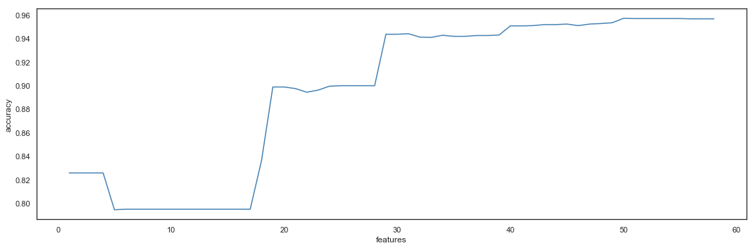
accuracies_smote.nlargest(10, 'accuracy')
| features | accuracy | cols | |
|---|---|---|---|
| 50 | 50 | 0.957111 | [Work_accident, promotion_last_5years, salary,... |
| 51 | 51 | 0.956889 | [Work_accident, promotion_last_5years, salary,... |
| 52 | 52 | 0.956889 | [Work_accident, promotion_last_5years, salary,... |
| 53 | 53 | 0.956889 | [Work_accident, promotion_last_5years, salary,... |
| 54 | 54 | 0.956889 | [Work_accident, promotion_last_5years, salary,... |
| 55 | 55 | 0.956889 | [Work_accident, promotion_last_5years, salary,... |
| 56 | 56 | 0.956667 | [Work_accident, promotion_last_5years, salary,... |
| 57 | 57 | 0.956667 | [Work_accident, promotion_last_5years, salary,... |
| 58 | 58 | 0.956667 | [Work_accident, promotion_last_5years, salary,... |
| 49 | 49 | 0.953333 | [Work_accident, promotion_last_5years, departm... |
The best model is found with 50 features, for an accuracy of 0.957.
logreg = LogisticRegression(solver='lbfgs', max_iter=250)
rfe_smote = RFE(logreg, accuracies_smote.nlargest(1,'accuracy').features.values.ravel()[0])
rfe_smote = rfe_smote.fit(os_data_X, os_data_y.values.ravel())

print(sum(rfe_smote.support_),'selected features:')
for i in list(os_data_X.loc[:, rfe_smote.support_]):
    print(i)
50 selected features:
Work_accident
promotion_last_5years
salary
department_IT
department_RandD
department_accounting
department_hr
department_management
department_marketing
department_product_mng
department_sales
department_support
department_technical
workload_extreme
workload_high
workload_normal
workload_very low
time_spend_company_cat_high departure
time_spend_company_cat_low departure
time_spend_company_cat_no departure
average_montly_hours_bin_(0, 125]
average_montly_hours_bin_(125, 131]
average_montly_hours_bin_(131, 161]
average_montly_hours_bin_(161, 216]
average_montly_hours_bin_(216, 274]
average_montly_hours_bin_(274, 287]
average_montly_hours_bin_(287, 310]
last_evaluation_bin_(0.00, 0.44]
last_evaluation_bin_(0.44, 0.57]
last_evaluation_bin_(0.57, 0.76]
last_evaluation_bin_(0.76, 1.00]
attitude_low performance
attitude_normal
attitude_unhappy
attitude_very happy
attitude_very unhappy
project_performance_normal
project_performance_very low
number_project_cat_extreme
number_project_cat_normal
number_project_cat_too high
number_project_cat_too low
satisfaction_level_bin_(0.00, 0.11]
satisfaction_level_bin_(0.11, 0.35]
satisfaction_level_bin_(0.46, 0.71]
satisfaction_level_bin_(0.71, 0.92]
satisfaction_level_bin_(0.92, 1.00]
efficiency_high
efficiency_low
efficiency_very low
The selected columns are really numerous compared to the initial dataset. However, the model is built to check its metrics.
cols_smote = list(os_data_X.loc[:, rfe_smote.support_])
os_data_X_sel = os_data_X[cols_smote]
X_smote_test_sel = X_smote_test[cols_smote]
cv_acc(lr, os_data_X_sel, os_data_y, 10, seed)
print()
lr_run(lr, os_data_X_sel, os_data_y, X_smote_test_sel, y_smote_test)
10-fold cross validation average accuracy: 0.962

Iteration  1 | Accuracy: 0.96
Iteration  2 | Accuracy: 0.95
Iteration  3 | Accuracy: 0.96
Iteration  4 | Accuracy: 0.95
Iteration  5 | Accuracy: 0.96
Iteration  6 | Accuracy: 0.95
Iteration  7 | Accuracy: 0.97
Iteration  8 | Accuracy: 0.97
Iteration  9 | Accuracy: 0.97
Iteration 10 | Accuracy: 0.97

Accuracy on test: 0.957

              precision    recall  f1-score   support

           0       0.98      0.97      0.97      3435
           1       0.90      0.92      0.91      1065

   micro avg       0.96      0.96      0.96      4500
   macro avg       0.94      0.95      0.94      4500
weighted avg       0.96      0.96      0.96      4500

Confusion Matrix:
[[3322  113]
 [  80  985]]

                                  Feature      Coef.
0                              intercept.  17.376456
1                           Work_accident  -1.540492
2                   promotion_last_5years  -0.877758
3                                  salary  -0.827350
4                           department_IT  -3.555270
5                        department_RandD  -3.633989
6                   department_accounting  -3.178568
7                           department_hr  -2.706043
8                   department_management  -3.374921
9                    department_marketing  -3.230675
10                 department_product_mng  -3.256803
11                       department_sales  -3.244566
12                     department_support  -2.799412
13                   department_technical  -2.786458
14                       workload_extreme   1.262675
15                          workload_high  -1.314907
16                        workload_normal  -2.114032
17                      workload_very low  -2.160452
18  time_spend_company_cat_high departure  -2.366082
19   time_spend_company_cat_low departure  -3.898360
20    time_spend_company_cat_no departure  -4.220065
21      average_montly_hours_bin_(0, 125]  -2.160452
22    average_montly_hours_bin_(125, 131]  -1.748431
23    average_montly_hours_bin_(131, 161]  -2.290330
24    average_montly_hours_bin_(161, 216]  -2.490469
25    average_montly_hours_bin_(216, 274]  -2.054918
26    average_montly_hours_bin_(274, 287]  -1.536961
27    average_montly_hours_bin_(287, 310]   1.262675
28       last_evaluation_bin_(0.00, 0.44]  -1.708380
29       last_evaluation_bin_(0.44, 0.57]  -2.715554
30       last_evaluation_bin_(0.57, 0.76]  -2.290356
31       last_evaluation_bin_(0.76, 1.00]  -3.664226
32               attitude_low performance  -1.708380
33                        attitude_normal  -1.835470
34                       attitude_unhappy  -2.648314
35                    attitude_very happy  -3.123197
36                  attitude_very unhappy   1.817110
37             project_performance_normal  -1.234341
38           project_performance_very low  -1.708380
39             number_project_cat_extreme   1.958954
40              number_project_cat_normal  -3.429596
41            number_project_cat_too high  -2.845605
42             number_project_cat_too low  -3.041480
43    satisfaction_level_bin_(0.00, 0.11]   1.817110
44    satisfaction_level_bin_(0.11, 0.35]  -1.231504
45    satisfaction_level_bin_(0.46, 0.71]  -2.114606
46    satisfaction_level_bin_(0.71, 0.92]  -1.447229
47    satisfaction_level_bin_(0.92, 1.00]  -3.145082
48                        efficiency_high   1.124227
49                         efficiency_low   1.463810
50                    efficiency_very low  -3.650808
plot_roc(lr, X_smote_test_sel, y_smote_test)

The model run on over-sampled dataset has an accuracy really closed to the model run on the original dataset. We can conclude that the imbalanced proportions of the target in our dataset didn’t insert bias in our model.
However, as more variables are necessary to achieve an equivalent accuracy, it indicates that the feature selection might have been biased by our feature construction. In fact, the binned features were built to fit the data, and allow to remove many features from our initial model. But this technique makes our model over-fit the data, reducing its chances to achieve the same accuracy with a new dataset. This might explain why the Recursive Feature Elimination cannot select the same features:
list_features = pd.DataFrame({'Initial':sorted(list(accuracies.loc[accuracies.features == 14]['cols'])[0]),
                          'SMOTE':sorted(list(accuracies_smote.loc[accuracies_smote.features == 14]['cols'])[0])})
list_features
| Initial | SMOTE | |
|---|---|---|
| 0 | attitude_normal | attitude_normal |
| 1 | attitude_unhappy | attitude_very happy |
| 2 | attitude_very happy | average_montly_hours_bin_(287, 310] |
| 3 | attitude_very unhappy | department_IT |
| 4 | average_montly_hours_bin_(287, 310] | department_RandD |
| 5 | efficiency_low | department_accounting |
| 6 | efficiency_very low | department_management |
| 7 | number_project_cat_extreme | department_marketing |
| 8 | satisfaction_level_bin_(0.00, 0.11] | department_sales |
| 9 | satisfaction_level_bin_(0.92, 1.00] | department_technical |
| 10 | time_spend_company_cat_no departure | efficiency_very low |
| 11 | time_spend_company_cat_very high departure | satisfaction_level_bin_(0.00, 0.11] |
| 12 | workload_extreme | satisfaction_level_bin_(0.92, 1.00] |
| 13 | workload_normal | time_spend_company_cat_no departure |
However, the model can be tested using the exact same selection of columns than the ones selected by the initial RFE.
cols_1 = cols.copy()
cols_1.remove('left')
print(cols_1)
os_data_X_sel_1 = os_data_X[cols_1]
X_smote_test_sel_1 = X_smote_test[cols_1]
['workload_extreme', 'workload_normal', 'time_spend_company_cat_no departure', 'time_spend_company_cat_very high departure', 'average_montly_hours_bin_(287, 310]', 'attitude_normal', 'attitude_unhappy', 'attitude_very happy', 'attitude_very unhappy', 'number_project_cat_extreme', 'satisfaction_level_bin_(0.00, 0.11]', 'satisfaction_level_bin_(0.92, 1.00]', 'efficiency_low', 'efficiency_very low']
cv_acc(lr, os_data_X_sel_1, os_data_y, 10, seed)
print()
lr_run(lr, os_data_X_sel_1, os_data_y, X_smote_test_sel_1, y_smote_test)
10-fold cross validation average accuracy: 0.937

Iteration  1 | Accuracy: 0.95
Iteration  2 | Accuracy: 0.93
Iteration  3 | Accuracy: 0.95
Iteration  4 | Accuracy: 0.93
Iteration  5 | Accuracy: 0.94
Iteration  6 | Accuracy: 0.94
Iteration  7 | Accuracy: 0.94
Iteration  8 | Accuracy: 0.93
Iteration  9 | Accuracy: 0.93
Iteration 10 | Accuracy: 0.93

Accuracy on test: 0.938

              precision    recall  f1-score   support

           0       0.98      0.94      0.96      3435
           1       0.83      0.94      0.88      1065

   micro avg       0.94      0.94      0.94      4500
   macro avg       0.90      0.94      0.92      4500
weighted avg       0.94      0.94      0.94      4500

Confusion Matrix:
[[3224  211]
 [  69  996]]

                                       Feature     Coef.
0                                   intercept.  0.698509
1                             workload_extreme  1.946942
2                              workload_normal -1.989443
3          time_spend_company_cat_no departure -2.883204
4   time_spend_company_cat_very high departure  2.039475
5          average_montly_hours_bin_(287, 310]  1.946942
6                              attitude_normal -2.701934
7                             attitude_unhappy -1.732064
8                          attitude_very happy -2.828182
9                        attitude_very unhappy  2.587483
10                  number_project_cat_extreme  3.936500
11         satisfaction_level_bin_(0.00, 0.11]  2.587483
12         satisfaction_level_bin_(0.92, 1.00] -2.878639
13                              efficiency_low  2.863472
14                         efficiency_very low -4.951222
The resulting accuracy is still really good, which confirms that the initial model didn’t have bias due to the imbalance of the dataset.
The high accuracy is anyway driven by the binned features tailored to the dataset. If they work really well for this data, it might not be the case for another dataset. The features should instead be set using standard binning approach, which wouldn’t fit as well the data but which would be adaptable to any dataset. That solution would be recommended if the model has to be run in production.